Model fitting

Fitting models to data

$$ \newcommand{\L}{\mathcal{L}} $$

Motivation

A powerful approach to theory-data integration is the use of statistical methods that directly combine empirical data with the mechanistic models of theoretical ecology. This is the world of model-fitting.

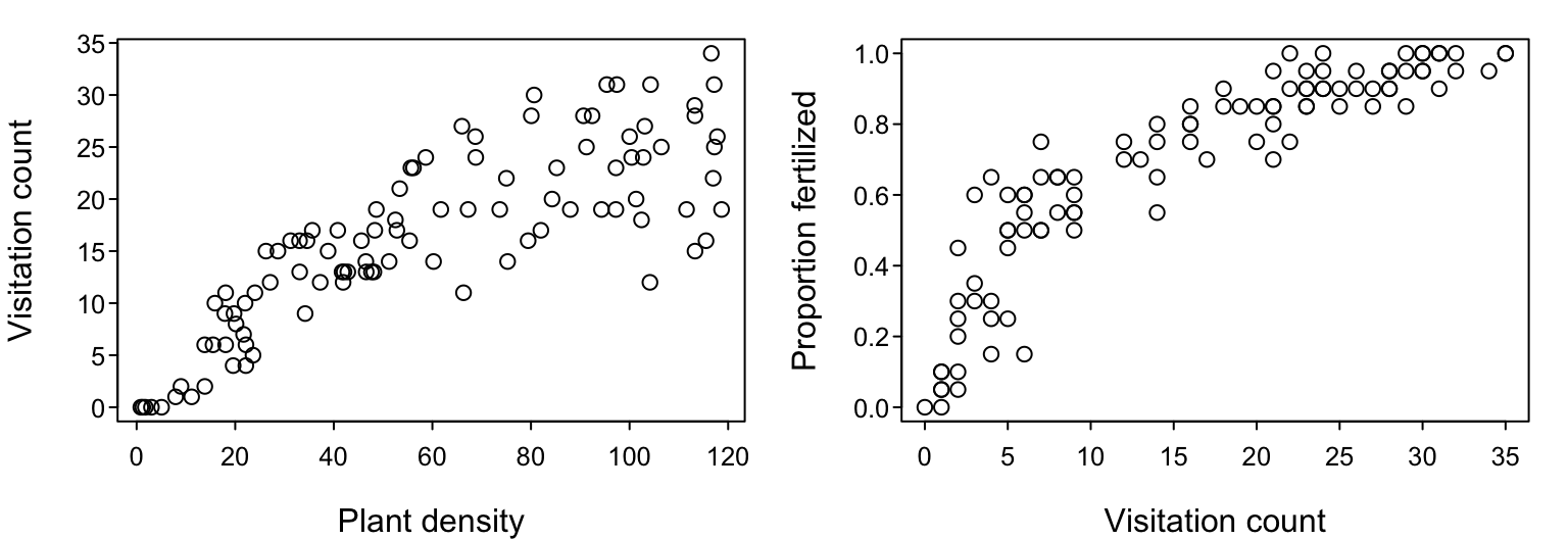
Perhaps we performed a study in which we counted the number of pollinator visits the flowers of a focal plant species received over a range of different plant densities and now wish to characterize the relationship between these variables. (To keep things simple, we’ll assume each plant has only a single flower.) Or perhaps we performed an experiment in which we varied the number of pollinator visits that the flowers of the plant species received and are now interested in characterizing how this variation in visits influenced ovule fertilization success (i.e. the proportion of ovules in each flower that were successfully fertilized).

In the past, the common way to characterize any such relationship among variables was to use linear or non-linear least-squares regression (including polynomial regression), extending more recently to mixed effects models. Generalized linear models and generalized additive models have also become popular, largely because they can accommodate non-Gaussian error structures and flexible, non-linear relationships.

But these types of statistical models are generally not “mechanistic”; their functional forms are not derived from “first-principles” ecological theory. Instead, these types of models are by and large only “descriptive” in nature.

Theoreticians, on the other hand, have derived many non-statistical (deterministic) mathematical equations to encapsulate how different biological processes should/could influence the patterns we see in nature. Our goal is to develop the skills to (1) fit such mechanistic models to data in order to obtain best-fitting parameter estimates while accommodating process-appropriate error structures, and (2) compare the relative performance of several such models in order to identify those that perform best at representing the data.

We will achieve these things using the principle of maximum likelihood and an information-theoretic model-comparison approach. Other approaches for model fitting and comparison — such as Bayesian statistics — are often used to accommodate complex data structures and for other pragmatic and epistomological reasons, but those are beyond what we will cover. That said, most of the principles that we will cover are directly relevant to these other approaches as well.

Overview

To understand the principle of maximum likelihood, we first need to understand some fundamentals regarding probability distributions and likelihood functions. We’ll then see how theory models can be incorporated into likelihood functions to convert them from deterministic models to statistical models. It’s this conversion that permits us to fit them to data. We will then develop our intuition for maximum likelihood parameter estimation (i.e. model fitting) by first doing it analytically and then learning to use numerical optimization.

Having fit several models to a dataset, we will then dip our toes into the methods of comparing their relative performance using information criteria.

Skip down to the end result to see where we’re headed.

Required R-packages

In principle, everything we’ll discuss can be accomplished using functions that come pre-loaded in base R, but we’ll make use of the bbmle package for a few conveniences at the very end.

# install.packages('bbmle', dependencies = TRUE) # use to install if needed
library(bbmle)

## Loading required package: stats4

Exercise code

In addition to the in-text links below, you can download what you’ll need in this GoogleFolder.

Fundamentals

We’re going to start by assuming our focal response variable doesn’t vary in response to any possible covariates at all. Doing so is useful in helping us think about the different types of probability distributions there are, and which may be best in representing the type of stochastic processes that are likely to have generated our data.

Probability distributions

Our two example data sets above share some things in common because they both represent (or are derived from) counts of things. Counts are integer-valued (i.e. 0, 1, 2, 3, …) and can’t be negative. The proportion of fertilized ovules is derived from two counts: the count of fertilized ovules and the total count of available ovules. Count data are a very common type of data in ecology, so we’ll focus on them for our purposes.

Among the simplest and most appropriate probability distributions to represent such data are the Poisson and binomial probability distributions. Because they represent counts, they are discrete distributions.

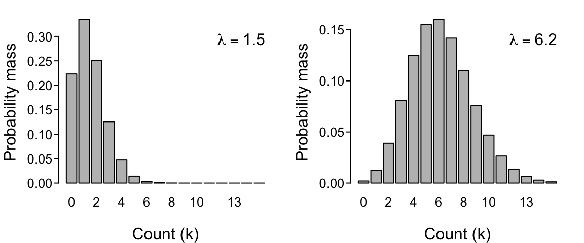
The Poisson distribution

The Poisson distribution would be appropriate for our dataset in which the count of visitations is our response variable. It is written as $$ Pr(k|\lambda) = \frac{\lambda^k e^{-\lambda}}{k!} $$ and expresses the probability that $k$ events will occur in some interval of time (i.e. that the count of events will be equal to $k$) given that the process responsible for generating the events occurs at a constant mean rate $\lambda$. You can read $Pr(k|\lambda)$ as the probability of $k$ events given parameter $\lambda$. The symbol $e$ represents an exponential (i.e. Euler’s number: 2.718…) and the symbol $!$ represents the factorial function (e.g., $4! = 4 \times 3 \times 2 \times 1$).

Below, with data on replicate counts of $k$, we will presume that the Poisson applies and then estimate the value of parameter $\lambda$ that is most likely to have generated those counts. Intuitively, a higher underlying value of parameter $\lambda$ will result in higher $k$ counts when we draw from this distribution repeatedly (i.e. when we obtain samples from the data-generating process). In fact, $\lambda$ reflects the count that we expect to observe on average across many such draws (a fact that we will prove later).

The Binomial distribution

The binomial distribution would be appropriate for our dataset in which the proportion of fertilized ovules is our response variable. More specifically, it will be appropriate after we re-express the number of counts (number of fertilized ovules) expected under the binomial distribution as a proportion of the maximum number of counts possible (the total number of ovules in a flower). The binomial is written as $$ Pr(k, n|p) = {n \choose k} p^k (1-p)^{n-k} = \frac{n!}{k!(n-k)!} p^k (1-p)^{n-k} $$ and expresses the probability of observing $k$ events in a total of $n$ tries given that each event either does or does not happen with constant probabilities $p$ and $1-p$ respectively.¹ The first part of the equation, ${n \choose k}$, is read as “$n$ choose $k$”. For example, given $n$ available ovules in a flower, $k$ of them are successfully pollinated. (The proportion $k/n$ thus corresponds to our measure of fertilization success.) The larger the probability $p$ of success and the larger the number of $n$ tries, the larger that the average count of $k$ successes will be over replicate samples from the data-generating process.

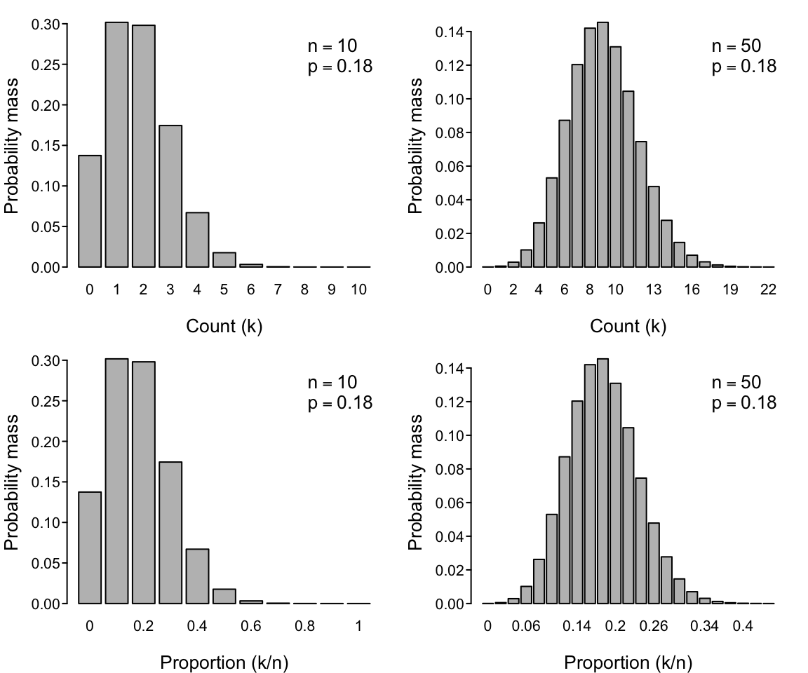
Note that in contrast to the Poisson distribution where the potential count $k$ could be arbitrarily high, $k$ is bounded by the maximum possible value of $n$ under the binomial distribution. Although the average process rate is assumed constant under both distributions, a flower can be visited many times ($k \geq 0$), making the Poisson more appropriate. On the other hand, an ovule that has already been fertilized can’t be fertilized again (thus $0 \leq k \leq n$), making the binomial more appropriate for our second experiment.

Other probability distributions

There are dozens of probability distributions available, but the Poisson and binomial are arguably the simplest and most useful (and thus among the most commonly assumed in ecology). One reason for this is that they have only a single free parameter ($\lambda$ and $p$, respectively) given that $n$ is usually known. These parameters determines not only the expected (mean) value of the distribution of the $k$ counts but also their variance. (For the Poisson, both the mean and the variance equal $\lambda$, while for the binomial the mean is $np$ and the variance is $np(1-p)$.)

Other distributions allow the mean and the variance to be separated. For example, the negative binomial and beta-binomial are discrete examples that generalize the Poisson and binomial distributions to accommodate the common occurrence of over-dispersion (e.g., a variance that is larger than the mean).

Another distribution that you’re probably much more familiar with is the Normal (a.k.a. Gaussian) distribution. The Normal distribution has two parameters $\mu$ and $\sigma$ that respectively determine its mean and variance. The Normal distribution has a long history of use in ecology and statistics, and is a biologically-appropriate distribution in many circumstances (thanks to the power of the Central Limit Theorem). It could even be appropriate in the circumstances of our two example data sets because both the Poisson distribution and the binomial distribution converge on the Normal distribution (see the figures above). But that is only true for sufficiently large $\lambda$, and sufficiently large $n$ and intermediate $p$, respectively.

In our context of “mechanistic” models, we often have data from situations where the conditions that lead to a Normal distribution are far from satisfied. For example, when flower abundances are very low, visitation rates ($\lambda$) will be very low. For small $\mu$ and large $\sigma$, the Normal distribution will also give negative values, which often don’t make sense for ecological data sets (you can’t have negative counts). Finally, in the context of fitting mechanistic models, we often don’t care about estimating the variance; our goal is typically to estimate the parameter values that maximize a model’s fit to the mean of our data. In that sense, having an extra variance parameter, such as $\sigma$ of the Normal distribution, is actually a nuisance (they’re often called “nuisance parameters”) because it means the model is more complex and thus potentially more challenging to fit. Just as (or even more) importantly, these nuisance parameters can lead to biased estimates of the other “mechanistic” parameters that we actually do care about, especially when sample sizes are not large (as is often the case in Ecology).

Likelihood functions

Probability distributions express the probability of an outcome given their parameter(s). For the Poisson distribution we therefore wrote $Pr(k, n | \lambda)$, but more generically for any discrete distribution we’ll write $Pr(y | \theta)$, using $y$ to represent outcomes and $\theta$ the parameter(s). $Pr(y | \theta)$ is referred to as a probability mass function; the input is the parameter values in $\theta$ and the output is the probability of any potential outcome $y$.

In contrast, when we have data and want to estimate the parameters of a presumed model, we want the reverse. We then talk of wanting to quantify the likelihood of any potential parameter value given the data. We therefore write $\L(\theta | y)$. $\L(\theta | y)$ is referred to as the likelihood function; the input is an outcome and the output is the likelihood that a potential parameter value could have generated that outcome.

If we observe a given outcome then the most likely parameter value to have generated that outcome is the one that maximizes the probability of the outcome. We therefore define the likelihood function to be the probability mass function, setting $$ \L(\theta | y) = Pr(y | \theta). $$ This may seem silly, but it’s a conceptually important step.

Assuming the Poisson specifically, we therefore have $$ \L(\lambda | k) = Pr(k | \lambda) = \frac{\lambda^k e^{-\lambda}}{k!}. $$

The method of maximum likelihood is a matter of finding the value of the parameter that will maximize the output of the likelihood function when we input observed outcomes.

Note on discrete vs. continuous probability distributions.

Maximum likelihood

Intuition

As just stated, maximum likelihood estimation is a matter of the finding the value of the parameter(s) that maximize the likelihood of having observed our data. Let’s walk through how we would do that, first assuming we have only a single data point and then assuming we have many.

Single observation

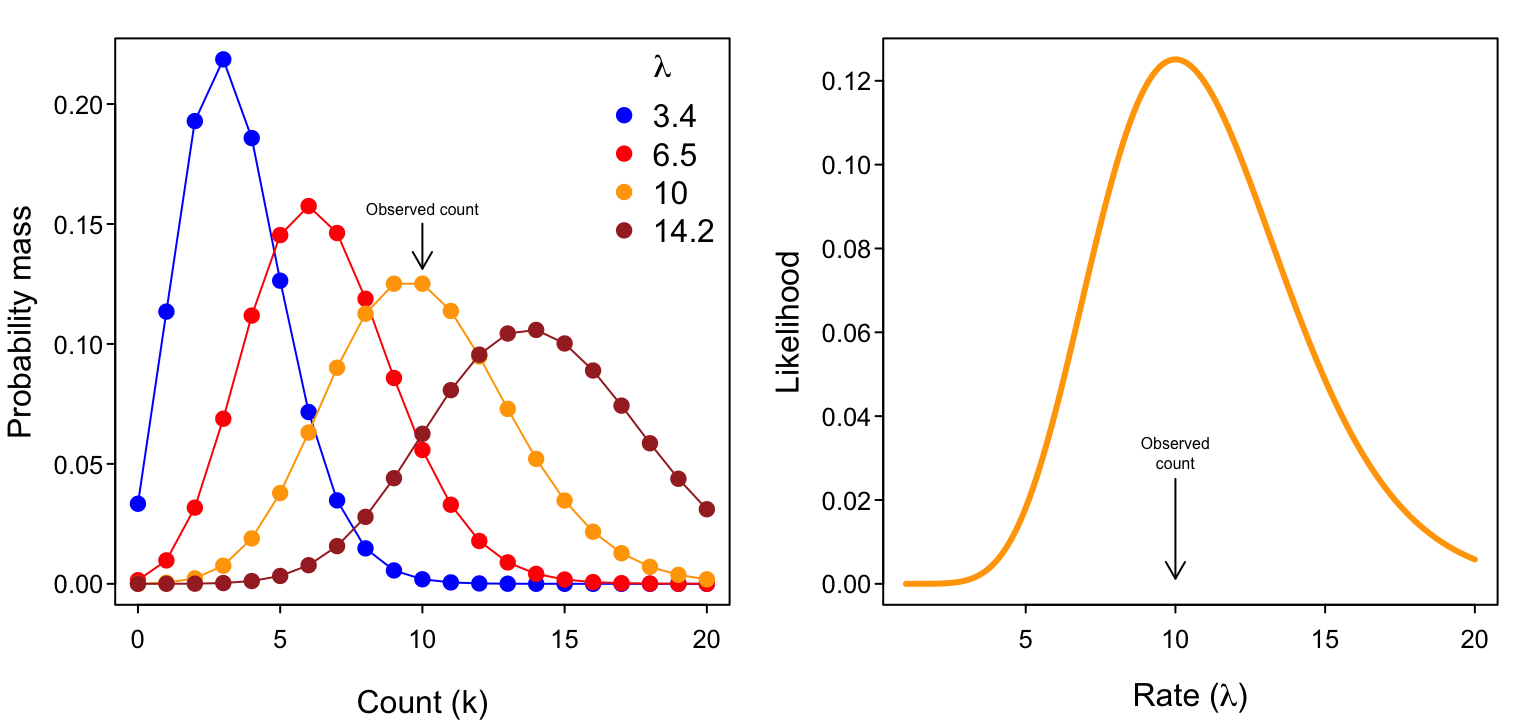
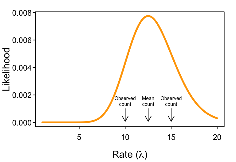
Let’s say that we sat in a meadow, watched a single flower for some amount of time, and observed a total of $k=10$ pollinator visits in that time. Presuming the Poisson to be an appropriate representation of the visitation process, we can use our data to determine the most likely value for $\lambda$.

Remember that $\lambda$ reflects the underlying visitation rate (visits per time) of the process and then think about the following plots of

• the probability mass $Pr(k | \lambda )$ as a function of potential $k$ values (with our data $k=10$ highlighted) for various values of $\lambda$, and
• the likelihood $\L(\lambda | k)$ as a function of $\lambda$ for $k=10$.

Notice that the illustrated likelihood function on the right has a maximum at a count of exactly $k=10$.² That is, given our observation of $k=10$ visits, the most likely value of the rate parameter $\lambda$ is 10. (Hopefully that’s not all too surprising; remember that $\lambda$ reflects the expected (mean) value of a Poisson-distributed variable.)

Multiple observations

What do we do when we have not just one but multiple observations? That is, what if we had a field assistant who also watched a single flower and counted $k=15$ visits in the same amount of time? We therefore have two observations, $k = {10, 15}$, to consider.

If the probability of the first observation is $Pr(k=10 | \lambda)$ and the probability of the second observation is $Pr(k=15 | \lambda)$, then the probability of observing both is their product, $Pr(k={10, 15} | \lambda) = Pr(10 | \lambda) \cdot Pr(15 | \lambda)$.

The same is true for likelihoods. To get the overall (“joint”) likelihood of $\lambda$ given both observations, we simply multiply their likelihoods. Thus $\L(\lambda | k={10, 15}) = \L(\lambda | k=10) \cdot \L( \lambda | k=15)$. More specifically, $$ \L(\lambda | k={10, 15}) = \frac{\lambda^{10} e^{-\lambda}}{10!} \cdot \frac{\lambda^{15} e^{-\lambda}}{15!}. $$ As the next figure shows, $\L{\lambda | k={10, 15})$ has a maximum at $\lambda = 12.5$ (which corresponds to the average of the two observations).

For an arbitrary number of $n$ observations (i.e. $k={ k_1, k_2, \ldots, k_n}$), we have a product of $n$ observation-specific likelihoods. Our joint likelihood function with which to determine $\lambda$ thus becomes a function of these observation-specific likelihoods, $$ \L(\lambda |k) = \prod_{i=1}^n \frac{\lambda^{k_i} e^{-\lambda}}{k_i!} $$ where the symbol $\prod_{i=1}^n$ denotes the product of elements $i=1$ to $n$. That is, $$ \prod_{i=1}^n \frac{\lambda^{k_i} e^{-\lambda}}{k_i!} = \frac{\lambda^{k_1} e^{-\lambda}}{k_1!} \cdot \frac{\lambda^{k_2} e^{-\lambda}}{k_2!} \cdot \ldots \cdot \frac{\lambda^{k_n} e^{-\lambda}}{k_n!}. $$

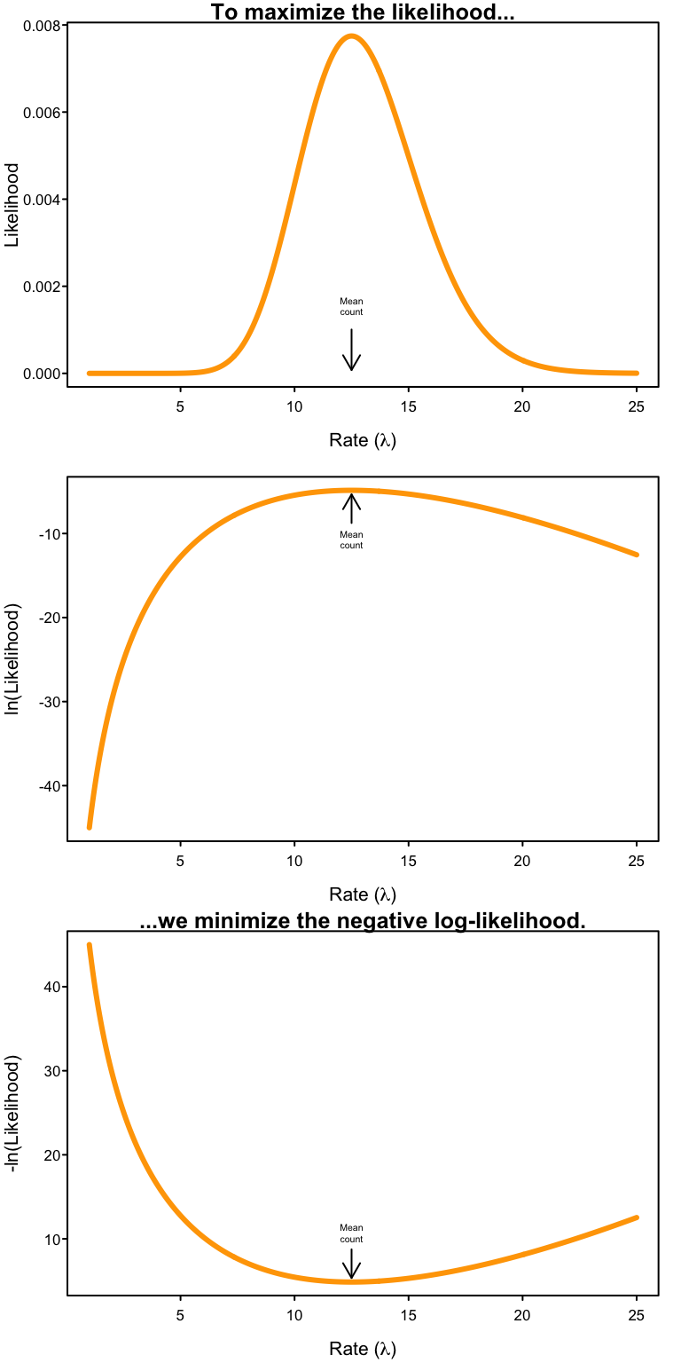
Why the negative log-likelihood?

We want the value of $\lambda$ that maximizes the joint likelihood over all our observations. But we’ve created a numerical problem in the previous step. Probabilities are numbers bounded by 0 and 1, and therefore so are likelihoods. As a result, by multiplying all those likelihoods together, our joint likelihood will become a smaller and smaller number with every data point we add to our dataset! In fact, as our number of observations grows their joint likelihood becomes a vanishingly small number that neither our heads nor computers can deal with!

The solution is the logarithm.³ Processes that are multiplicative on the natural scale become additive on the logarithmic scale, i.e. $$ \ln ( x\cdot y \cdot z) = \ln(x) + \ln(y) + \ln(z). $$ Therefore, $$ \ln \L(\lambda |k) = \ln \left (\prod_{i=1}^n \frac{\lambda^{k_i} e^{-\lambda}}{k_i!} \right) = \sum_i^n \ln \left (\frac{\lambda^{k_i} e^{-\lambda}}{k_i!} \right) $$ where $$ \sum_i^n \ln \left (\frac{\lambda^{k_i} e^{-\lambda}}{k_i!} \right) = \ln \left(\frac{\lambda^{k_1} e^{-\lambda}}{k_1!} \right ) + \ln \left( \frac{\lambda^{k_2} e^{-\lambda}}{k_2!} \right) + \ldots + \ln \left (\frac{\lambda^{k_n} e^{-\lambda}}{k_n!} \right ). $$ Thus the log-likelihood increases (rather than decreases) in value as the number of observations increases. Big numbers are no problem to deal with, so we’ve successfully avoided our numerical problem.

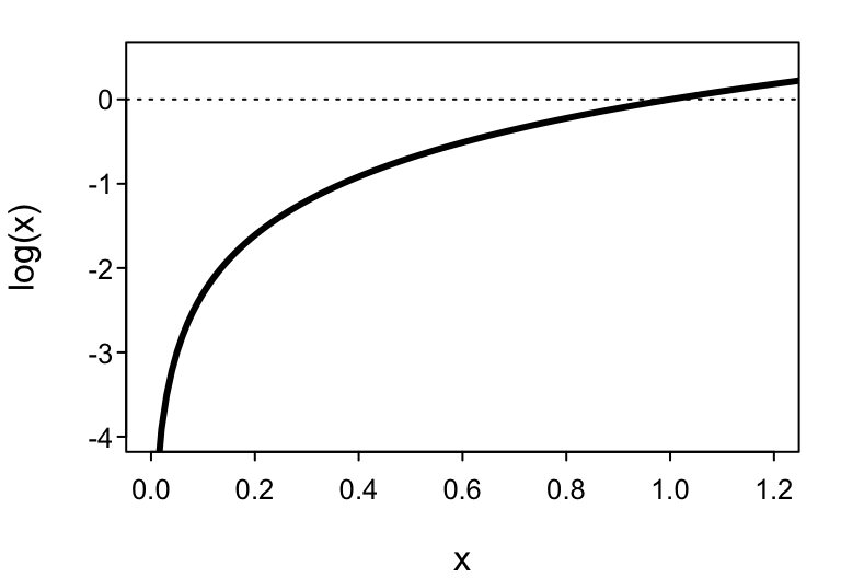
But taking the logarithm has a side effect because the logarithm of a number between 0 and 1 returns a negative number. Since each of the individual likelihoods is between 0 and 1, a side-effect of taking $\ln \L$ is that we’re now adding up lots of negative numbers. That’s not a problem because we can just take the negative log-likelihood to get back to a positive number. But importantly, as a consequence, in order to maximize the likelihood $\L$, we need to minimize the negative log-likelihood $-\ln \L$ to find the parameter value that best fits the data.

Finding the MLEs

For some models it is possible to determine the values of the parameters that maximize the likelihood function analytically. That is, it’s possible to solve for the maximum likelihood parameters (i.e. the maximum likelihood estimators (“MLEs”)). Doing so for $\lambda$ of the Poisson, we can (i) build intuition to better understand what numerical methods (“optimizers”) are about, and (ii) prove that the MLE for $\lambda$ of the Poisson is the mean of the $k$ observations (as I simply proclaimed above). However, I’ll relegate the latter of these to the Of Potential Utility or Interest page.

Analytical intuition

We’ll do this rather abstractly…

Suppose we have some arbitrary function, like this polynomial describing a parabola $f(x) = a + b (x-c)^2$ depicted in the following figure. The way to find the value of $x$ where $f(x)$ is at its minimum value is to find the value of $x$ where the slope of $f(x)$ (with respect to $x$) is zero.

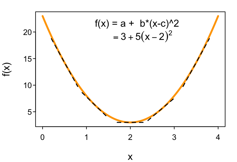
How do we determine the slope of $f(x)$ as a function of $x$? We take the derivative of $f(x)$ with respect to $x$: $\frac{d ; f(x)}{dx}$. For our polynomial, $\frac{d ; f(x)}{dx} = 2b(x-c)$, which even R has the ability to solve symbolically:

D(expression(a + b * (x-c)^2), 'x')

## b * (2 * (x - c))

Setting $\frac{d; f(x)}{dx} = 2b(x-c) = 0$ (since that’s where $f(x)$ will have its minima (or maxima)⁴), we use a little algebra to solve for $x$: $$ 2b(x-c)=0 \implies 2bx-2bc=0 \implies 2bx = 2bc \implies x=c $$ (which correctly equals the location of the minimum at $x=2$, as shown in the above figure). We can do the same thing for likelihood functions to obtain their MLEs. Doing so often leads to useful insight into the processes and variables that cause parameter estimates to change in value.

Numerical optimization

There are two basic parts to finding the MLE by numerical means: coding the negative log-likelihood function and choosing the optimization method to find its minimum.

Coding the likelihood

For the Poisson, we have the negative log-likelihood function

$$ -\ln \L(\lambda | k) = \sum_i^n \ln \left (\frac{\lambda^{k_i} e^{-\lambda}}{k_i!} \right). $$ You could certainly write code to define an R function to implement this calculation (see the Of Potential Utility or Interest page), and sometimes it’s necessary to do that for more complex likelihoods. But R has built-in functions for most probability distributions that are robust, fast, and easy to use. These R functions are the “density functions” of the probability distributions.

For example, while R’s function runif(n, min, max) draws n random values from the uniform probability distribution bounded by min and max parameter values, the corresponding density function dunif(x, min, max) returns the likelihood of the value x given min and max. For the Poisson, we have dpois(x, lambda).

Note that, by default, the likelihood is returned on the natural scale. To obtain the negative log-likelihood of x, we use -dpois(x, lambda, log = TRUE).

When x represents a vector of values (multiple observations), we obtain a vector of corresponding negative log-likelihoods (one for each observation). Since we want the overall joint negative log-likelihood of all the observations, we have to sum their negative log-likelihoods together: -sum(dpois(x, lambda, log = TRUE)). We can define our own R function to implement this and use it more conveniently. Notice that we define the function with only lambda as an argument.

# Define the negative log-likelihood
nlL.pois <- function(lambda){
  -sum(dpois(k, lambda, log = TRUE))
}

Continuing with our dataset of $k = {10, 15}$ observations from above, we can apply our function as follows:

# Define k globally for our nlL.pois() function to use.
k <- c(10, 15)

# Demonstrate use of nlL.pois() for two hypothetical values of lambda.
nlL.pois(11)

## [1] 5.056302

nlL.pois(12.4)

## [1] 4.861272

Optimization

Given data $k={10, 15}$, we now need to find the value of $\lambda$ that minimizes our negative log-likelihood function nlL.pois(). For many circumstances, the R function optim() is the go-to function for doing so because it is robust and has several standard optimization methods and control options to choose from. It comes in base R, so there’s no package to load.

At minimum, we have to pass optim(par, fn, ...) where fn is the function we wish to minimize and par is a guess at an initial parameter value at which the optimizer will start its search. (You can ignore the warning message in the following example.⁵)

init.par <- list(lambda = 2)
optim(init.par, nlL.pois)

## Warning in optim(init.par, nlL.pois): one-dimensional optimization by Nelder-Mead is unreliable:
## use "Brent" or optimize() directly

## $par
## lambda 
##   12.5 
## 
## $value
## [1] 4.860468
## 
## $counts
## function gradient 
##       34       NA 
## 
## $convergence
## [1] 0
## 
## $message
## NULL

The output of optim() includes the MLE for our parameter $\lambda$, the value of our negative log-likelihood function at the MLE, and a convergence error code (with 0 indicating success).

Let’s try it

Repeat for yourself

In-class 10-15 minutes

Download ModelFitting_1.R to implement what we just did with the $k={10, 15}$ data set and Poisson distribution. Then try generating different data sets that vary in their sample size to see how close you get to the true value of $\lambda$ with which you generated the data. (We’ll address estimation uncertainty through the use of confidence intervals later.)

Real binomial data

Your actual challenge, however, is to generate your own data and write your own code to analyse it.

The data set will be contributed to by everyone in the class. Each of you will take one (or more) Delphinium seed pods and count both the total number of ovules and the number that were successfully fertilized. Enter your data on this GoogleSheet.

As soon as you’re done with data entry, download the data as a csv file and start analyzing it. (You can re-download it again after everyone’s finished entering their data. You only need one data point to start fitting this one-parameter model!)

Rather than using a Poisson, you’ll want to assume a binomial process. Your goal is to estimate $p$, the average probability of fertilization success. Download ModelFitting_2.R to help you get going.

Model fitting

Up to this point, we have assumed that the process that is reflected in our data, be it the flower visitation rate $\lambda$ or the fertilization success probability $p$, is well-represented as being a constant value that is independent of any other contributing factor. Visually, if we actually had data like that introduced at the very start of today, our models so far would correspond to the horizontal lines in the following figures. That is, we’d be assuming that visitation counts are independent of plant density, and that the proportions of ovules fertilized are independent of visitation count. All variation is noise.

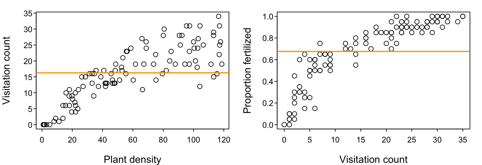
We can think of these models of constant $\lambda$ and $p$ as being our simplest 1-parameter “null” models; if you didn’t have any other information, your best prediction for the expected value of a future data point would be the mean of current data. Clearly, these data visualizations indicate that these null models do not capture all the information that a more complex model could potentially capture. Although there is plenty of noise, the visitation rate and the fertilization success probability appear to be increasing functions of plant density and visitation count, respectively. That is, $\lambda$ would probably be better considered to be a function of plant density and $p$ would probably be better considered to be a function of visitation count. So how do we go about encoding that in our models?

Well, there are many ways that we could do it. We could go the route of using GLMs and GAMs that permit us to continue to appropriately represent non-Gaussian error structures and potentially non-linear relationships (see the Of Potential Utility or Interest). But, as motivated above, our goal is to fit mechanistic models instead.⁶

Mechanistic models

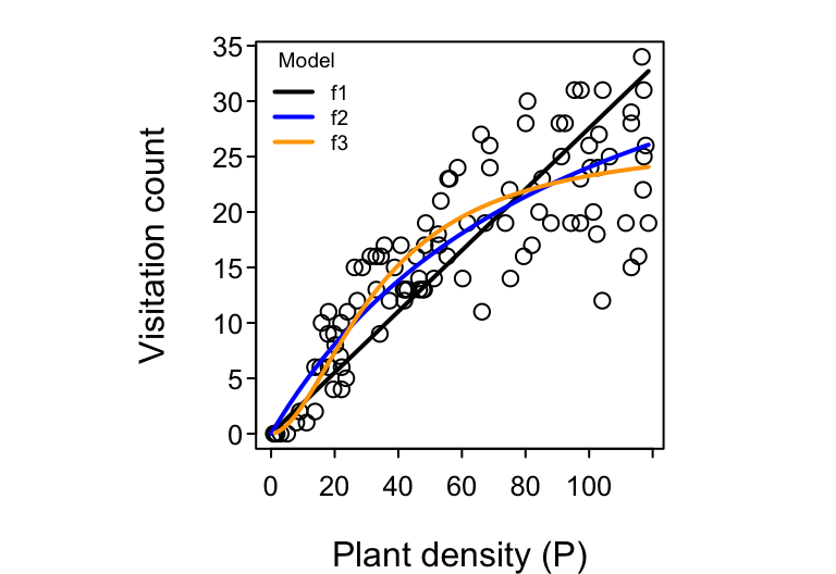
Let’s consider our visitation count vs. plant density dataset. Even if the total number of pollinators that are flying in the sky is invariant (constant) with respect to the density of our focal plant species, it seems somewhat intuitive that we should see more total visits to the focal plant in areas where the focal plant’s density is higher. That is, setting aside targeted searching and all other kinds of potential pollinator behavior, it should be true that the more plants there are, the greater the chance that a pollinator will bump into any one of them by random chance alone. The mathematically simplest model, we’ll call it $f_1$, to describe such a presumed dependence of $\lambda$ on $P$ would be $$ \text{Visitation rate }\lambda = f_1(P) = a P, $$ where a new parameter $a$ encapsulating what may potentially be several aspects of the pollinator’s search effort, including its flying speed, its preference for the focal plant, etc.. The higher the value of $a$, the steeper the slope of the assumed biological relationship between $\lambda$ and $P$ and hence the steeper the slope of observed visitation counts versus plant density we expect to see in our data. In the literature on Consumer-Resource theory, this model is referred to as the Holling Type I functional response.⁷

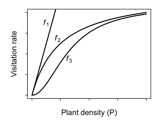
A more flexible (and possibly more realistic) second model describes $\lambda$ as increasing with $P$ in a monotonically-saturating fashion to encode the hypothesis that visitation rates can’t increase with $P$ forever. That is, while visitation rates are likely determined by search effort and plant density at low $P$ (just like for model $f_1$), they are probably bounded at some maximum possible visitation rate at high values of $P$. If, for example, a pollinator spends $h$ minutes per visit to each encountered flower, then the maximum possible visitation rate at high values of $P$ (where there is effectively no time needed to search and find the next flower) is $1/h$ visits per minute. The two-parameter model $$ \text{Visitation rate }\lambda = f_2(P) = \frac{a P}{1 + a h P} $$ encapsulates this. The more plants there are, the more that each pollinator spends time “handling” rather than searching and encountering more plants. In the literature, this model is referred to as the Holling Type II functional response. (An alternative but deterministically-equivalent parameterization is referred to as the Michaelis-Menten model.) Note that when $h=0$, model $f_2$ collapses back to model $f_1$. Model $f_1$ is therefore nested within $f_2$.

Lastly, an even more flexible (and possibly even more realistic) third model describes $\lambda$ as increasing with $P$ in a sigmoidal fashion to encode the hypothesis that a pollinator’s search rate may additionally be limited at low $P$. For example, the rate at which a pollinator searches for plants may itself increase with plant density; they may develop an ever better “search image” as they encounter more plants. The three-parameter model $$ \text{Visitation rate }\lambda = f_3(P) = \frac{a P^\theta}{1 + a h P^{\theta}} $$ encapsulates this when the new parameter $\theta$ (theta) takes on values greater than 1. This model is most appropriately referred to as the Holling-Real Type III functional response.⁸ Note that when $\theta=1$, model $f_3$ collapses back to model $f_2$ since $x^1 = x$.

Modifying the likelihood

To fit the three $f_1-f_3$ models to our data we need to incorporate them into our likelihood function. To do so we insert each of them in for $\lambda$. Many refer to the resulting statistical model (i.e. the likelihood function) as being composed of a deterministic skeleton and a stochastic shell. For example, for model $f_1$ we have $$ -\ln \L_1(a | k, P) = \sum_i^n \ln \left (\frac{f_1^{k_i} e^{-f_1}}{k_i!} \right) = \sum_i^n \ln \left (\frac{(a P)^{k_i} e^{-a P}}{k_i!} \right). $$ Notably, unlike our original negative log-likelihood function to which we supplied only the response variable data (visitation counts $k = {k_1, k_2, \ldots, k_n }$) in order to estimate the constant $\lambda$, we must now supply the both response variable data and the covariate data (of corresponding plant densities $P = {P_1, P_2, \ldots, P_n }$) in order to estimate up to three constants ($a$, $h$, and $\theta$) for the three models.⁹ But because $P$ is the same for all models, we can just leave it defined in R’s global environment (rather than defining it within the function’s internal environment).

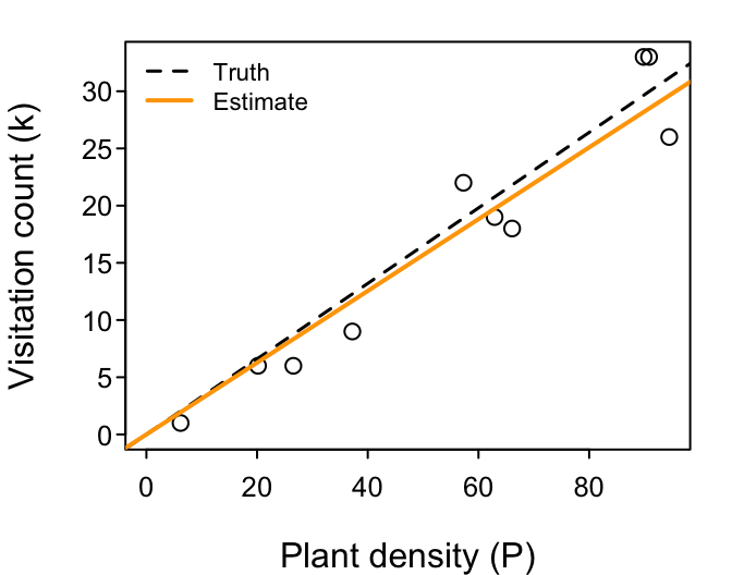
We’ll need a little more dummy data, so let’s create it using runif() and rpois():

set.seed(1)

a <- 0.33 # True value of 'a'
n <- 10 # Sample size
P <- runif(n, 0, 100) # Plant densities
k <- NULL # Visitation counts
for(i in 1:n){
  k[i] <- rpois(1, a * P[i]) # Generate a k for each P assuming Type 1
}
print(data.frame(P = round(P, 1), k))

##       P  k
## 1  26.6  6
## 2  37.2  9
## 3  57.3 22
## 4  90.8 33
## 5  20.2  6
## 6  89.8 33
## 7  94.5 26
## 8  66.1 18
## 9  62.9 19
## 10  6.2  1

Now we define the negative log-likelihood for the $f_1$ and use optim() to estimate the MLE for its $a$ parameter. (Again we’ll ignore the warning for this 1-dimensional model.)

nlL.pois.f1 <- function(par){
  a <- par['a']
  -sum(dpois(k, a * P, log = TRUE))
}

# Estimate 'a'
fit <- optim(par = list(a = 0.2),
             fn = nlL.pois.f1)

## Warning in optim(par = list(a = 0.2), fn = nlL.pois.f1): one-dimensional optimization by Nelder-Mead is unreliable:
## use "Brent" or optimize() directly

print(fit) 

## $par
##         a 
## 0.3136914 
## 
## $value
## [1] 24.37161
## 
## $counts
## function gradient 
##       28       NA 
## 
## $convergence
## [1] 0
## 
## $message
## NULL

# True 'a'
print(a)

## [1] 0.33

# Estimated 'a'
fit$par

##         a 
## 0.3136914

Let’s try it

Repeat for yourself

In-class 30-45 minutes

Download ModelFitting_3.R. The first part generates a random dataset. It then repeats the fitting of the $f_1$ model that we just did.

Your challenge is expand on the script to fit the $f_2$ and $f_3$ models to the same dataset. Summarize what you learn by comparing the three models' (1) parameter MLEs to each other and the values with which the dataset was generated, and (2) their minimized negative log-likelihoods (i.e. the value of their negative log-likelihood at their parameter MLEs). Which model’s parameters got closest to the truth? Which model is the best-fitting? (Is it a higher or a lower negative log-likelihood that is better?) Which model is the best-performing?

But before you get going, take note of two things about

1. Coding the likelihood, and
2. Initial values & NaNs.

Coding the likelihood

The function we used to define the negative log-likelihood for the $f_1$ model above had only a single par argument from which we “extract” parameter a using a <- par['a']. (That is, we’ve added a line of code relative to what we did when we were just focused on $\lambda$.) You’ll want to do the same thing when defining the likelihood functions for models $f_2$ and $f_3$; your likelihood functions must have only one par argument from which each parameter is extracted.

Initial values & NaNs

In general, the more data you have and the simpler the model, the less sensitive the optimization will be to your initial parameter value guess. In our simple example case involving $f_1$ and a linear relationship, almost any reasonable initial value for $a$ would have worked.

In slightly more complex cases, you can often get a good enough guess by eyeballing your data and thinking about how the parameters of your deterministic function should influence its shape. For example, for the $f_2$ model, parameter $a$ controls the slope at the origin at $P=0$ while parameter $h$ controls the level of the asymptotic maximum value of $1/h$ as $P\rightarrow \infty$, both of which can be read of a plot of the data. Otherwise, the best way to proceed is to fit a simpler model and to use its MLEs to inform your guess for the next more complex model. (That is, fit $f_1$ first and use its estimate for $a$ to inform the initial value for $a$ in model $f_2$, etc.)

In complex cases, it’s often wise to try out several different starting values to ensure that you always arrive at the same MLE values. Otherwise you run the risk of your optimizer finding a local (rather than global) minimum in the likelihood surface (see below).

You may get a negative log-likelihood output of NaN if your initial guess (or a value attempted during the optimization) is incompatible with the data. optim() will tell you when that happens. If that happens for the initial value, try again with a different value. If it happens during the optimization, it’s typically not a problem if a convergence code of 0 is obtained.

Model comparison

In general, the more parameters a model has (i.e. the more parametrically complex it is), the better it will fit the data. Indeed, a little simplistically speaking, if you have a model that has as many free parameters as you have data points, then your model can fit the data perfectly with no unexplained residual variation leftover!¹⁰ A model’s fit to the data as reflected by its likelihood (or its $R^2$ value) is thus rarely useful on its own when we want to compete different models against each other to ask which is “the best”. Rather, the principle of parsimony (Occam’s razor) motivates us to identify the best-performing model. Typically the best-performing model is the one that maximizes fit while minimizing complexity relative to the other considered models. If two models fit the data equally well but one uses fewer parameters to achieve that fit, then it is the better-performing model. Currently, the most widely used tools for quantifying relative model performance are based on information theory.

AIC & BIC

Two information-theoretic indices of model performance are by far the most popularly used in ecology: the Akaike Information Criterion (AIC) and the Bayesian Information Criterion (BIC, a.k.a. the Schwartz Information Criterion). The practical difference between these three criteria is in how they quantify model complexity.

The AIC score of a model is calculated as twice the minimized negative log-likelihood plus twice the number of parameters $p$: $$ AIC = - 2 \ln \hat{\L} + 2 p. $$ Note two things:¹¹

1. We’re using the modified symbol $\hat{\L}$ rather than just $\L$ to indicate that we are using the minimized value of negative log-likelihood (i.e. its value at the model’s parameter MLEs).
2. Because a lower $-\ln \hat{\L}$ value reflects a better fit to the data, adding a model’s parameter count with $+2p$ reflects a complexity penalty that makes a model’s AIC value larger.

Similarly, the $BIC$ score of a model is calculated as

$$ BIC = - 2 \ln \hat{\L} + \ln(n) p, $$ where the logarithm of the dataset’s sample size $n$ also contributes to the complexity penalty term. Therefore, larger datasets impose a greater penalty on more parametrically-complex models for BIC.

For both criteria, the model with the lowest score is considered the best-performing model. Note that when comparing models the dataset cannot change. All models have to be fit to the same dataset. More specifically, although the covariates can be different for different models, the response variable data (e.g., our visitation counts) must remain the same.

Relative performance

Having identified the best-performing model, it is natural to ask just how much better the best-performing model is relative to the others. We can do that by calculating their $\Delta$ differences. That is, the performance of the $i^{th}$ model relative to the best performing model is calculated as $$ \Delta_i = AIC_i - AIC_{min}. $$ The best-performing model will thus have $\Delta_i = 0$ and all others will have $\Delta_i > 0$. The bigger the difference, the better the best-performing model. Because we like cut-offs¹², by rule-of-thumb convention, a difference of at least 2 units is deemed to reflect “substantial” support in favor of the best-performing model, a 2-4 unit difference is deemed as providing “strong” support¹³, a 4-7 unit difference as “considerably less” support, while models having $\Delta_i > 10$ are deemed to have essentially no support.

Let’s try it

In-class 10-15 minutes

Adding to your updated copy of ModelFitting_3.R, write functions for $AIC$ and $BIC$ and use them to identify the best-performing model among our three $f_1$ - $f_3$ models. Do your inferences differ from your earlier evaluation of the models?

Alternatives

Information criteria like AIC and BIC are popular because they are super easy to implement. They also have the benefit of enabling the comparison of any set of models for which a likelihood can be calculated and the parameters can be counted (or estimated). In particular, the models in the set need not be nested subsets of each other as is necessary for the alternative model-comparison approach of Likelihood Ratio Tests. (Our $f_1$ - $f_3$ models are nested subsets, because $f_3$ can be reduced to $f_2$ which can be reduced to $f_1$, so likelihood ratio tests could be used.)

There are also several other information criteria available. The commonly-used AICc attempts to account for a bias towards more complex models that occurs for AIC when sample sizes are small. For models that are linear in their parameters and have residuals that are well-approximated by a Normal distribution, $$ AIC_c = AIC + \frac{2k(k+1)}{n-k-1}. $$ Unfortunately there is no similarly simple equation for nonlinear models with non-Normal residuals.

Other approaches for balancing fit and complexity include the Fisher Information Approximation (FIA) which considers not just a model’s parametric complexity but also its geometric complexity (i.e. how flexible it is), and various forms of cross-validation whereby subsets of a given data set are repeatedly left out of the fitting (“training”) process to be used as “test data” with which to evaluate the model’s predictive ability. In the latter, unnecessarily complex models will over-fit the training data and will therefore perform poorly on the test data.

Philosophies

Much has been written about the pros and cons, foundations and assumptions, epistomological and pragmatic differences between the various approaches to model comparison. That’s particularly true for AIC vs. BIC. The comparison is often framed as being rather absolute and clear (especially in the ecological literature), but my sense is that it is far more nuanced and muddy.

Much of the discussion pertains to questions of motivation in comparing alternative models. Is it to describe your data? Is it to predict new data? Is it to explain your data? If it’s to predict, then what kind of prediction are you wanting to make (e.g., within-sample, out-of-sample, out-of-range, forecast, etc.)? Conceptually, all questions will arrive at the same conclusion regarding which model is “best” when your data set is very large and sufficiently representative of all possibilities, but that is rarely if ever the case. Therefore, choices about which approach to take have to be made. For example, the derivation of AIC is motivated by a desire to maximize out-of-sample predictive ability (i.e. minimizing the prediction error when predicting what equivalent data sets would look like). Asymptotically (as sample sizes increase), AIC is equivalent to the leave-one-out form of cross-validation. In contrast, the derivation of BIC is motivated by a desire to identify the “true” model (i.e. to interpret or draw inferences about biology), and in that sense are more similar to leave-many-out forms of cross-validation and asymptotically converge on criteria like FIA.

That said, most of the mathematical and statistical basis for contrasting the different approaches is limited to linear regression type models. Thus, while I consider it important to go beyond what most ecologists seem to be doing (i.e. ignore the differences and just go with AIC because everyone else is using it) by thinking about your motivations and the trade-offs among them, I would say that a fair degree of pragmatism remains warranted.

Uncertainty

Likelihood surfaces

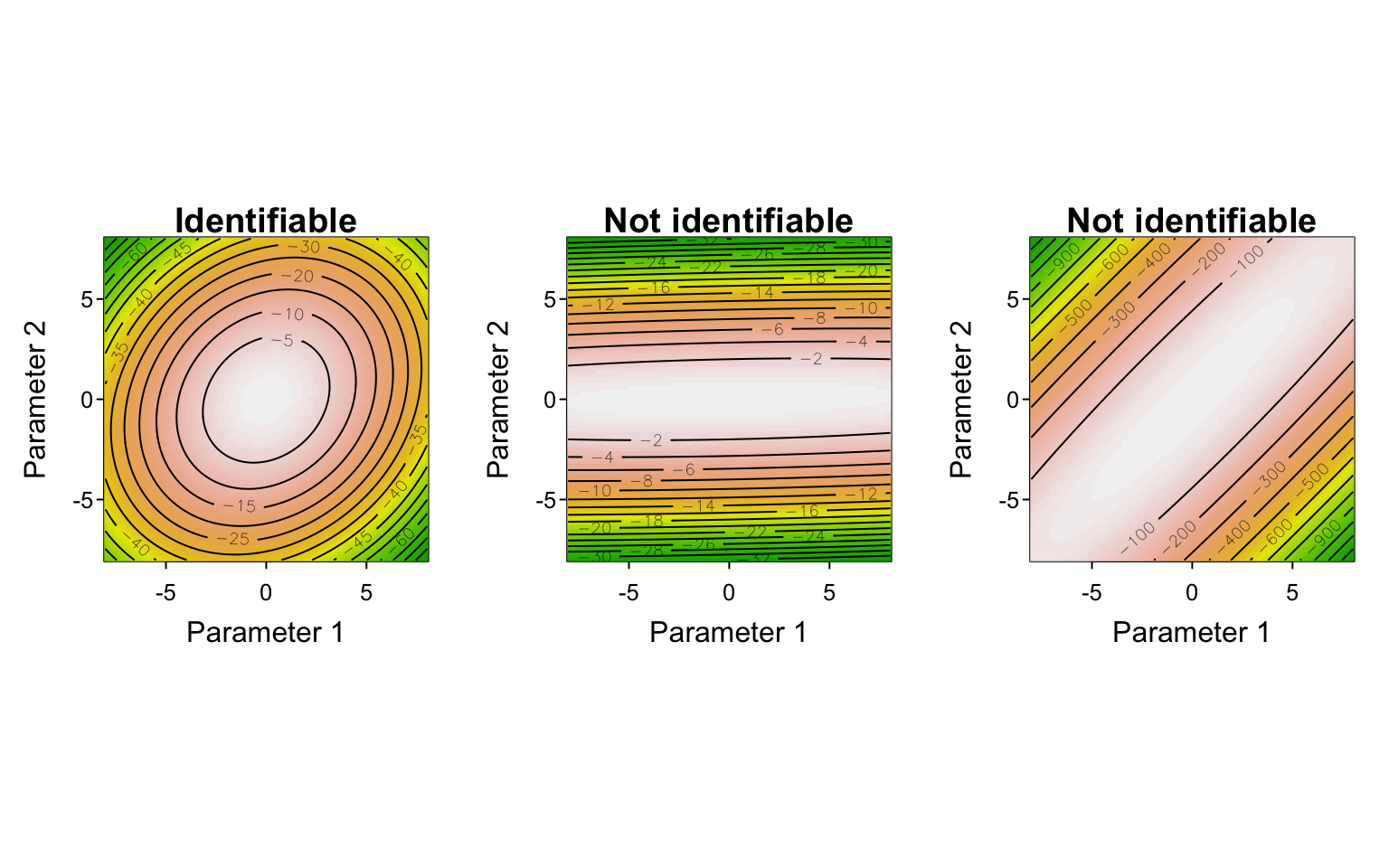
When we have more than one parameter, we talk about the likelihood function as describing a “likelihood surface”. For a model with 2 parameters, we can easily visualize that surface in a single plot. When a model has $p$ parameters there are $p$ dimensions to the likelihood surface. Minimizing the negative log-likelihood to obtain the parameter MLEs is equivalent to finding the lowest point of that surface. Doing so is not a problem when the surface is like a smooth, unimodal, round bowl shape with only one well-defined minimum point, but such a shape is far from guaranteed for all models and datasets. In fact, depending on the data and/or the model, a likelihood surface could exhibit many shapes that are different from that of a (multidimensional) bowl.

The shape of the likelihood surface relates to issues of parameter- (and model-) identifiability, and to attempts to quantify parameter uncertainty.

Identifiability

The likelihood surface could be wavy and have multiple minima. In that case our optimizer could potentially get stuck in a local minimum, unable to find the true MLE associated with the global (lowest) minimum. Different optimizers attempt to deal with this potential problem in different ways, but as alluded to above, it is often wise to start at different initial parameter values to confirm convergence to the same optimum.

The surface could be relatively flat in one or more parameters. The reasons for this include that there may be insufficient information in the data to constrain the values of the parameter(s) (i.e. all values are similarly likely); a parameter’s MLE would thus come with large uncertainty.

The surface could be relatively or even entirely flat for some combination of parameters. This could happen because the model (or the data) are structured in such a way that two or more parameters are not (sufficiently) identifiable. That is, parameters (or covariates) may co-vary in such a way that their independent effects cannot be distinguished. In two-dimensions, this would look like a likelihood surface that has a valley running through it. Each individual parameters apparent MLE could thus appear to be well-constrained (i.e. appear to have low uncertainty), but there could nonetheless be considerable uncertainty in their values.

My sense is that likelihood surfaces with multiple minima most commonly occur for datasets that are too small for the task. For small data sets, noise predominates and different parameter combinations fit different data points similarly well.

Flat surfaces or surfaces with valleys, on the other hand, will not be resolved simply by having more data (if it is similar to the data already available). Rather, what is typically needed is either more information and/or an alternatively formulated model structure. More information can come from better-designed ’experiments’ that, for example, (i) increase the range of values that the predictor variables exhibit (e.g., beyond what is “natural”), and (ii) increase the independence (decreases the co-variation) among predictor variables. Examples of alternative model structures include (i) replacing two parameters that always co-occur as a product by a single compound parameter, and (ii) rewritting a model in a mathematically equivalent (but statistically non-equivalent) formulation (e.g., the Holling Type II versus the Michaelis-Menten models). That said, these are relatively extreme, simple examples that represent a range of potential issues and solutions relating to identifability that you may encounter and where expert experience is often required.

Quantifying uncertainty

When our goal is to make comparisons of model performance using information criteria, then all we need from model fitting are the values of each model’s minimum negative log-likelihood associated with their parameter MLEs. However, many times we’re not only interested in just doing model comparison or just obtaining the MLE values of the parameters. Rather, we often would also like to characterize the statistical uncertainty (“clarity”) of the parameter estimates. The most common way to do that is by determining the 95% confidence intervals of the MLEs.

For that, we’ll make use of the mle2() and confint() functions from the bbmle package. mle2() uses optim() as the default optimizer to determine the parameter MLEs, and confint() takes the result and returns the parameter confidence intervals.

We’ll continue on with the small $n=10$ dataset we generated when we demonstrated the fitting of the $f_1$ model.

print(data.frame(P = round(P, 1), k))

##       P  k
## 1  26.6  6
## 2  37.2  9
## 3  57.3 22
## 4  90.8 33
## 5  20.2  6
## 6  89.8 33
## 7  94.5 26
## 8  66.1 18
## 9  62.9 19
## 10  6.2  1

library(bbmle)

nlL.pois.f1.bbmle <- function(a){
  -sum(dpois(k, a * P, log = TRUE))
}

fit <- mle2(nlL.pois.f1.bbmle, 
            start = list(a = 0.2))
print(fit)

## 
## Call:
## mle2(minuslogl = nlL.pois.f1.bbmle, start = list(a = 0.2))
## 
## Coefficients:
##         a 
## 0.3136831 
## 
## Log-likelihood: -24.37

confint(fit)

##     2.5 %    97.5 % 
## 0.2692366 0.3627788

Notice that

• mle2() wants the negative log-likelihood function to have (all) the parameters as arguments (unlike optim() which wanted a single par argument containing the parameters);
• mle2() has the order of the arguments for the negative log-likelihood and the list of initial parameter values reversed relative to optim(); and
• mle2() returns the (positive) log-likelihood rather than the negative log-likelihood. (I don’t know why.)

The bbmle package also has several other potentially useful functions that we won’t get into. Note that the above code is included at the bottom of ModelFitting_3.R.

End result

We used our visitation count data (introduced at the very start) to fit three models relating visitation rates to plant density. These models had either one, two, or three biologically-reasoned parameters that enabled the models to describe different types of relationships between observed visitation counts and plant density: linear, saturating, and sigmoid. The three models therefore reflected different expectations/hypotheses about the deterministic biological processes that could have generated the data, but in fitting them we also attempted to stay true to the likely stochastic processes that introduced noise to the data.

The results of our efforts are as follows:

We obtained maximum likelihood point estimates and their 95% confidence intervals for each of the three models.

## [1] "f1 parameters"

##  est.a  2.5 % 97.5 % 
##  0.276  0.262  0.289

## [1] "f2 parameters"

##     est 2.5 % 97.5 %
## a 0.485 0.412  0.576
## h 0.021 0.016  0.026

## [1] "f3 parameters"

##         est 2.5 % 97.5 %
## a     0.044 0.010  0.161
## h     0.038 0.031  0.043
## theta 1.812 1.385  2.310

Comparing the performance of the three models using AIC, we conclude that there is “substantial” support for model $f_3$ over the other two models.

##        AIC   dAIC  df
## fit.f3 538.4   0.0 3 
## fit.f2 552.0  13.6 2 
## fit.f1 613.1  74.7 1

Jump back to the Overview section.

Final thoughts

There is much that we have only touched on and even more we have swept under the rug, but hopefully we’re leaving you with a good enough starting point for your own interests. Most importantly, don’t get discouraged or frustrated by the challenge that model fitting can be. The process of model fitting has often been described as an “art”. It is a skill that is learned through practice and accumulated experience, and therefore through perseverance. And it’s worth pointing out that it’s a skill to be learned not only in regards to statistical and mathematical knowledge and comfort (e.g., experience with probability distributions and deterministic functions, respectively), but also in terms of empirical knowledge of the data and the biological (and data collection) processes that are likely responsible for having generated the data. Statisticians and mathematicians have just as hard a time thinking about biology as biologists do with the statistics and math! It’s in the challenge of gaining a balanced expertise in all three where the fun and excitement lies.

Readings

Aho, Derryberry, and Peterson (2014) Model selection for ecologists: the worldviews of AIC and BIC. Ecology, 95(3):631–636

Bolker (2008) Ecological models and data in R. Princeton University Press

Höge, Wöhling, and Nowak (2018) A primer for model selection: The decisive role of model complexity. Water Resources Research, 54(3):1688–1715

Murtaugh (2014) In defense of p values. Ecology, 95(3):611–617

Novak and Stouffer (2021) Geometric complexity and the information-theoretic comparison of functional-response models. Frontiers in Ecology and Evolution, 9:776

Novak and Stouffer (2021) Systematic bias in studies of consumer functional responses. Ecology Letters, 24(3):580–593

Solutions

ModelFitting_1.R (no ‘key’)

ModelFitting_2_key.R

ModelFitting_3_key.R

ModelFitting_4_key.R

Session Info

sessionInfo()

## R version 4.4.1 (2024-06-14)
## Platform: aarch64-apple-darwin20
## Running under: macOS Sonoma 14.5
## 
## Matrix products: default
## BLAS:   /Library/Frameworks/R.framework/Versions/4.4-arm64/Resources/lib/libRblas.0.dylib 
## LAPACK: /Library/Frameworks/R.framework/Versions/4.4-arm64/Resources/lib/libRlapack.dylib;  LAPACK version 3.12.0
## 
## locale:
## [1] en_US.UTF-8/en_US.UTF-8/en_US.UTF-8/C/en_US.UTF-8/en_US.UTF-8
## 
## time zone: America/Los_Angeles
## tzcode source: internal
## 
## attached base packages:
## [1] stats4    stats     graphics  grDevices utils     datasets  methods  
## [8] base     
## 
## other attached packages:
## [1] bbmle_1.0.25.1
## 
## loaded via a namespace (and not attached):
##  [1] cli_3.6.3           knitr_1.48          rlang_1.1.4        
##  [4] xfun_0.47           highr_0.11          jsonlite_1.8.8     
##  [7] htmltools_0.5.8.1   sass_0.4.9          rmarkdown_2.28     
## [10] grid_4.4.1          evaluate_0.24.0     jquerylib_0.1.4    
## [13] MASS_7.3-61         fastmap_1.2.0       mvtnorm_1.2-6      
## [16] yaml_2.3.10         lifecycle_1.0.4     numDeriv_2016.8-1.1
## [19] bookdown_0.40       compiler_4.4.1      rstudioapi_0.16.0  
## [22] blogdown_1.19       lattice_0.22-6      digest_0.6.37      
## [25] R6_2.5.1            bslib_0.8.0         Matrix_1.7-0       
## [28] tools_4.4.1         bdsmatrix_1.3-7     cachem_1.1.0