Networks

Analysis of structure

Motivation

Ecological networks offer a powerful approach to comprehensively analyze entire systems comprising hundreds of species and their thousands of interactions. There are almost infinite ways in which hundreds of species can possibly interact. Networks allow to determine the specific, non-random interaction structure that actually occur in nature of those almost infinite possibilities. These networks also allow the study of the interplay between structure and dynamics of complex systems of interacting species, shedding light on how this interplay influences system responses to perturbations.

Overview

Required R-packages

# PACKAGE LIST:
Packages <- c("tidyverse",
              "kableExtra",
              "bipartite") 

# (INSTALL AND) LOAD PACKAGES:
# install.packages(Packages, dependencies = TRUE)
lapply(Packages, library, character.only = TRUE)

Exercise code and data

In addition to the in-text links below, you can download what you’ll need in this GoogleFolder.

Terminology

A network consists of nodes and edges, where nodes represent discrete entities like people, computers, cities, or species, and edges (or links) represent the connections between these entities. Networks can be weighted or unweighted, depending on whether the connections have associated values or not. In weighted networks, the edges have numerical values that indicate the strength or distance of the connection between nodes. In the case of plant-pollinator networks, that weight has traditionally been the number or fraction of visits or pollen transported.

Networks can also be directed or undirected. In directed networks, such as food webs, the connections between nodes have a specific direction, such as the flow of energy, indicating a one-way relationship. In undirected networks, such as mutualistic networks, the connections are bidirectional, showing a two-way relationship between nodes (i.e., reciprocal benefits). We will see later that the reciprocal benefits between plant and pollinator species can be decomposed into the mechanisms by which those benefits are provided, which can convert the bidirectional links between species into two unidirectional links (i.e., consumption of floral rewards and pollination services).

Networks can also be unipartite or bipartite. Unipartite networks such as food webs consist of a single set of nodes (species), where edges can connect any pair of nodes within that set (any species can potentially be eaten by others). On the other hand, nodes in bipartite networks are divided into two disjoint sets, such as plants and pollinators, and edges (representing which pollinator species visits which plant species) only connect nodes from different sets (e.g., plants cannot visit other plants).

Below, there is an illustration of a plant-pollinator system represented as a bipartite network, with three plant and three pollinator species.

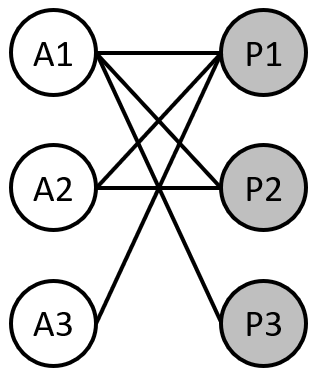
Ecological networks can be represented in various ways including a graph (as shown in the image above) or a matrix. Being able to switch between graph (network) and matrix form is powerful for understanding the full suite of network metrics we will see later.

Exercise 1

Using the bipartite network graph above, draw the corresponding matrix for the network. Assume that matrix columns represent animal species while matrix rows represent plant species. In the matrix cells, use 1’s to indicate an interaction between that animal and plant species and 0’s or blanks to indicate no interaction between species.

From data to networks

Two practical skills underpin everything on this page: converting empirical data into a bipartite matrix, and visualizing networks. Both are covered in the pre-workshop modules, and are not repeated here:

Prework – Edgelist-to-Network: turning an edge list (the usual field or metabarcoding data format) into a bipartite matrix with plants as rows and pollinators as columns, and getting it into the matrix form that the bipartite package expects (plant names as row names, numeric cells).
Prework – Network Visualization: network diagrams (plotweb()) and matrix depictions (visweb()), why the same network can be drawn in $R! \times C!$ different ways, and how “packing” a matrix (sorting rows and columns by degree) standardizes the depiction and makes nestedness visible.

From here on we assume your data are already in that standardized matrix form. The medgarden.csv dataset built in the Edgelist-to-Network prework is reused in an exercise below.

Metrics of structure

A useful summary of network metrics and their effect on network robustness to species extinctions can be found in this TedEd video: Valdovinos Ted Ed video

Connectance

Connectance measures the proportion of potential interactions that are realized in the network (i.e., the number of different interactions observed as a fraction of the total number of interactions that could possibly occur). Thus, connectance ranges between 0 (no connections between any species) and 1 (every species interacts with every other species). In unipartite networks, connectance is calculated by dividing the number of realized interactions (or links connecting species) $L$ by the square of the number of nodes $S$ in the network, which represents the total number of interactions if all species were fully connected to one another, including themselves. So, $C=L/S^2$. However, in a bipartite network, nodes from different sets cannot interact. Which should be the expression for connectance in a bipartite network?

Exercise 2

The denominator of the connectance formula represents the total number of possible interactions in the network, if all species were fully connected to one another. What is the total number of potential interactions in a bipartite network such as a plant-pollinator one?

Exercise 3

Calculate the connectance of the bipartite network graph from Exercise 1 using the formula you derived in Exercise 2.

Nestedness

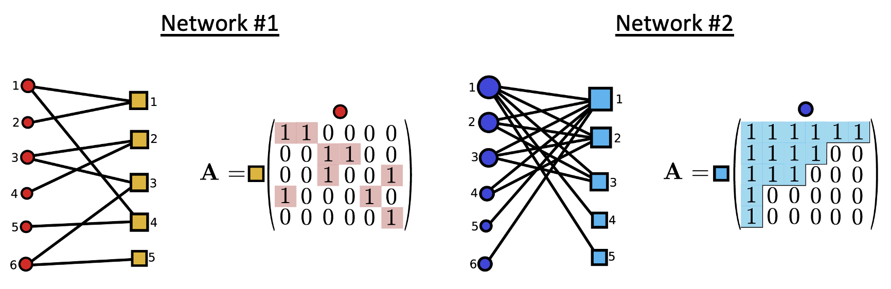
In a nested network, the interactions of the more specialized species are subsets of the interactions of the more generalized species. Another way to define nestedness is by saying that generalists tend to interact with both generalists and specialists while specialists tend to interact with mostly generalists. Note that the concept of specialist species in a network context is best interpreted as realized interactions and not necessarily as “true specialist” in the evolutionary sense. One particular species can be recorded as specialist (i.e., with only one interaction) in a particular day/week/season but then be recorded as a generalist in the next day/week/season.

Exercise 4

Given the two example networks below, which do you consider to have higher nestedness and why?

Modularity

A network is said to have high modularity when its interactions are compartmentalized into modules, whose species interact more among themselves than with species belonging to other modules.

Exercise 5

Given the two example networks of Exercise 4, which do you consider to have higher modularity and why?

Calculating metrics

We can calculate network metrics in empirical networks in a relatively straightforward way using the bipartite package for R. The networklevel() function calculates a huge number of different network metrics. This is not a function to use to spit out a zillion metrics and cherry-pick which ones look best—you will instead want to figure out a priori which metrics you are most interested in, and calculate only those.

For the “Safariland” plant-pollinator network dataset that comes included in the bipartite package, we can calculate nestedness with the NODF metric (there are many other ways to calculate nestedness):

networklevel(Safariland, 
             index = "NODF")

##    NODF 
## 24.5478

Easy! We can do the same thing for modularity (note: modularity can take some time to calculate, especially on older / slower computers):

networklevel(Safariland, 
             index = "modularity")

## modularity Q 
##    0.4301558

Exercise 6

Use the medgarden.csv data in matrix form, from the Edgelist-to-Network prework. Calculate:

$H_2’$ (network-level specialization); in networklevel, use index = "H2"
connectance

Relationships among metrics

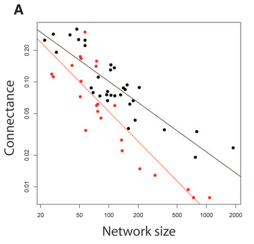
When analyzing the structure of a specific network and especially when comparing the structure of several networks, for example across a latitudinal or altitudinal gradient, you must keep in mind that all these metrics correlate, some positively others negatively. The best known of those relationships is the negative correlation between network richness (i.e., number of species) and connectance, which is shown in this image below taken from Thebault & Fontaine 2010 (Science), where species richness is labeled as “network size” and the black dots are mutualistic networks while the red dots are plant-herbivore bipartite networks.

Exercise 7

Given the mathematical formula of connectance, $C = L/(P \cdot A)$, how would you explain this well-known negative relationship between species richness, $S = P + A$, and connectance?

Other known relationships include the positive correlation between connectance and nestedness, the negative correlation between connectance and modularity, the positive correlation between species richness and nestedness, and the negative relationship between species richness and modularity.

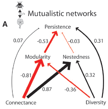
Understanding these relationships among network metrics is crucial when analyzing variations across environmental or perturbation gradients in network structure. For instance, if you are investigating how urbanization impacts the network structure of plant-pollinator communities and observe a significant negative impact of urbanization on species richness, caution is needed when comparing other network metrics across the urbanization gradient. This is due to the established relationship between species richness and various network metrics, which could potentially obscure the effect of urbanization by influencing connectance and modularity positively and nestedness negatively. That is, because decreased species richness increases connectance and modularity and decreases nestedness you may infer that it was urbanization which caused those effects on network structure but most likely it is the confounding effect of decreased species richness.

These correlations are exactly why comparing metrics between networks (across a gradient or a treatment) is hard, and why it needs its own approach—see Comparing networks, below. The short version: historically people used $z$-scores (an empirical metric standardized against its own null distribution) to make metrics comparable across datasets, but Song et al. (2017, Journal of Animal Ecology) showed the $z$-score itself depends on network size. Song et al. offered a replacement, but only for nestedness ($NODF_c$, via the maxnodf package; Hoeppke & Simmons 2021, Methods in Ecology and Evolution). The more general fix we cover below is downsampling.

Null models

In some situations, it is helpful to know if an empirical network exhibits a value of some network metric that is greater than you would expect by chance alone. Nestedness is a good example, because we might actually expect networks to display some level of nestedness just because of some of the basic facts of how they are set up. Most communities display a very skewed distribution of abundances, with one or just a few species having very high abundance, and then a lot of species with low abundances. If we have such an abundance distribution for both guilds (e.g. plant and pollinator species), and plants and pollinators are interacting with one another purely at random, we would expect that rare pollinator species would be most likely to interact with common plant species, and that rare plant species would be most likely visited by common pollinators. This is especially true if we are sampling the network on a per-area basis (in which we would log much more observation time on the most common plants). Taken together, the elements of this scenario—which with the exception of the random interactions, is pretty much the case in most plant-pollinator networks—would lead to a very nested pattern.

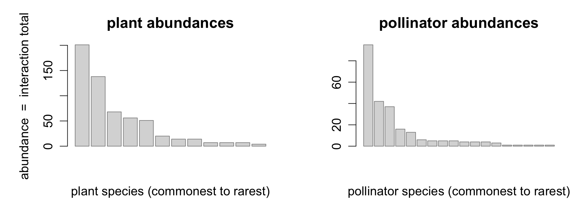
The two figures below make that concrete (they use the same code as the workshop presentation, with made-up data). First, a skewed abundance distribution for each guild—a few common species, many rare ones—treating each species’ abundance as its total number of interactions:

Now treat each species’ abundance as its interaction total, put those distributions on the margins of the plant-by-pollinator matrix, and fill the matrix by assigning interactions completely at random—each one to a plant and a pollinator with probability proportional to their abundances. Sorting rows and columns from commonest to rarest, common–common cells fill in and rare–rare cells stay empty:

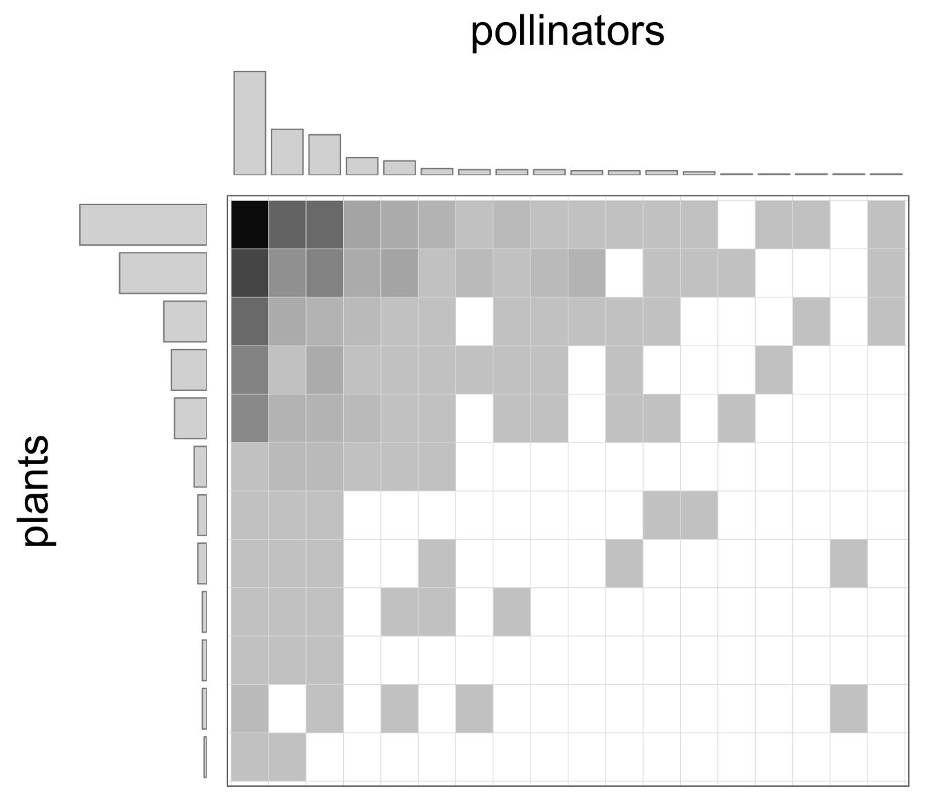
The result is a nested pattern that arose from abundances and random sampling alone, with no trait matching or other structuring mechanism. That is exactly why it is worth testing whether a real network is more nested than this.

Given that, we might ask if a network is more nested than we would expect it to be relative to chance alone. We can do this with null model simulations. What exactly is a null model? It’s a concept that has been surprisingly difficult to pin down, but the definition provided in the book “Null Models in Ecology” by Nick Gotelli & Gary Graves (1996, Smithsonian Institution Press, Washington, D.C.) is a helpful one:

“A null model is a pattern-generating model that is based on randomization of ecological data or random sampling from a known or imagined distribution. The null model is designed with respect to some ecological or evolutionary process of interest. Certain elements of the data are held constant, and others are allowed to vary stochastically to create new assemblage patterns. The randomization is designed to produce a pattern that would be expected in the absence of a particular ecological mechanism.”

If we were asking if a network is more nested than we would expect with chance alone, one way to frame that is to say that we don’t think interactions are happening randomly between plants and pollinators. Instead, plants and pollinators have traits that structure their interactions; pollinators draw down resource levels in flowers that then affect the preferences of other pollinators, etc. But, we can create a null model where we assume interactions are happening randomly, repeat that random interaction assignment many times, and then assess if our actual data are different (e.g., more or less nested) than we would expect based on random interactions. The basic statistical idea here is a permutation test, for those of you familiar with that concept.

Alternatives

But that sounds pretty complicated (and to be honest, it is not the most straightforward thing ever)—so how do we actually implement null models in practice? Luckily, the bipartite package has built-in algorithms to create null models (and there are other R packages that do as well, notably vegan), so you don’t have to code these by hand (phew!). But because there are different kinds of null models, it is critically important to understand what is going on “under the hood” of the algorithm so that you can apply the right null model to your analysis. Specifically, each algorithm holds certain features of the empirical network constant and lets the rest vary—and which features it holds constant determines which questions it can legitimately answer.

A quick terminology note, because the distinction matters a lot here:

a species’ degree is its number of interaction partners (how many species in the other guild it interacts with at least once)
a species’ marginal total (or interaction total) is its row or column sum—the number of interactions recorded for it, counting repeats

For a weighted network these are different numbers, and the common null-model algorithms preserve the marginal totals, not the degrees. (The workshop presentation and this page use “marginal total” / “interaction total” throughout for that reason.)

Simplest null model

Let’s start by thinking about the simplest possible way we could create a null model. We want to assume that interactions are happening at random. Perhaps a first-pass way of doing this would be to say something along the lines of “well we have our plant species and our pollinator species, i.e. our bipartite matrix, and we recorded a total of $N$ interactions in our empirical data… all we have to do is randomly assign each interaction to one cell in our bipartite matrix, and we’ll end up with a randomized network”. That would be one way to do it, but it has some pretty major downsides. One downside is that when you repeat that procedure, especially if your $N$ is relatively small, you are likely to have one or more species that have no interactions and thus would drop out of the network. Because some network metrics are sensitive (sometimes very sensitive) to network size / species richness, that’s definitely not ideal. You could get around that downside, perhaps by first assigning one interaction to each row (a random column in that row), and then assessing if all columns have an interaction, and for any that are missing, assigning a random interaction to that column. Then you could assign all of the “leftover” interactions randomly as described above.

Constant link number: `shuffle.web`

Making sure the species richness stays constant is an important improvement over the first-pass method, but the sketch of a null model described above still ultimately has some problems. One key reason is that while the number of total interactions is maintained, the sketch of the algorithm described above does not maintain the same number of links in the network. Given a wide-open matrix in which to assign interactions, in particular such an algorithm will typically generate many more links than we would see in an empirical dataset, and that is also definitely not ideal. A “second-pass” null model would maintain the same number of interactions (as we suggested in the “first-pass” model), but would also maintain the number of links (and therefore hold connectance constant). This is what the shuffle.web algorithm in the bipartite package does: it reshuffles all of the cell values across the matrix.

held constant: the grand total (number of interactions) and the number of filled cells—and therefore connectance
not held constant: the marginal totals (row and column sums)

Because the marginal totals are free to vary, shuffle.web tends to even them out: the common species no longer stay especially common. If you are testing nestedness, that means the null networks are typically less nested than a null that preserves the skew would be—so an empirical network is more likely to come out looking significantly nested. The same caveat applies to any metric that is sensitive to the skew in marginal totals.

shuffle.web has been used in some papers, e.g. Fortuna, M. A., and J. Bascompte. 2006. Habitat loss and the structure of plant-animal mutualistic networks. Ecology Letters 9: 281-286.

Constant marginal totals: `r2dtable`

Still, the shuffle.web null model algorithm is not widely used these days. A major reason is that (again) some plants, and some pollinators, are much more common, and some are rare. And that skewed abundance distribution could be a big driver of any nestedness we see in a system (as well as potentially other network metrics). To account for that, we can instead implement what we might call a “third-pass” algorithm that holds each species’ marginal total (row or column sum) constant. In practice, this would be straightforward to do for just one of the guilds in our network—let’s say we do it for plants. We can take the total number of interactions for each plant species, and assign them randomly across the pollinators in the network. Easy-peasy. The problem is that we are trying to do this also at the same time for pollinators, and that is a lot trickier! Again, luckily we don’t have to code this by hand. This null model is implemented in the r2dtable function in bipartite.

held constant: every row sum and every column sum (the marginal totals), and hence the grand total
not held constant: connectance (the number of filled cells)

This is essentially the null model implied by the skewed-abundance argument (and the figure) at the start of this section. It is the right choice if the metric you want to test with a null model is connectance. The downside is that connectance is free to move, and—as covered in Relationships among metrics—a shift in connectance drags nestedness, modularity, and specialization along with it. So if you are testing one of those, an r2dtable null can mislead. How can the row and column sums be fixed and yet connectance still change? The same marginal totals can be concentrated onto a few partners or spread across many; r2dtable draws tend to spread interactions out more than a real (often lopsided) network, raising connectance. The effect is small when the empirical margins are very constraining, larger in realistically-sized networks—worth checking if you use it.

Constant marginal totals and connectance: `swap.web`

Taking our exploration of null models yet another step further, r2dtable accounts for the number of interactions each species has, but does not give us back the same connectance as our data. So a “fourth-pass” algorithm holds both constant, relative to the empirical network:

held constant: the grand total (number of interactions), every marginal total (row and column sum), and connectance (the number of links)
not held constant: essentially only which cells the interactions land in, subject to the constraints above

This is implemented in the swap.web function in bipartite and is a very commonly-used null model. Because it is highly constrained, comparisons against it are more straightforward to interpret than comparisons against looser nulls. The flip side is that for small or highly structured networks there may be very few valid randomizations—in the extreme, a square network whose plant and pollinator marginal totals are both ${n, n-1, \dots, 1}$ has exactly one valid arrangement (perfectly nested). That is rarely an issue for empirical networks, but it is worth confirming your randomizations are actually distinct. This approach was first implemented in: Miklós, I. and Podani, J. (2004) Randomization of presence-absence matrices: comments and new algorithms. Ecology 85, 86–92.

There are other approaches as well, for example the vaznull function uses an approach proposed by Diego Vázquez et al. in 2007 (Oikos 116: 1120-1127). This algorithm weights the probability of selecting a cell (interaction) in the matrix by the abundance (number of empirically observed interactions) of both the plant and the pollinator. While similar to the r2dtable algorithm in that regard, it does not hold the row and column sums to be absolutely constant, even though they are weighted by interaction abundance. The vaznull algorithm is also supposed to maintain equal or close-to-equal connectance, like swap.web.

Comparing null models

Ultimately, however, it’s important to understand that every null model has drawbacks. In particular, more constrained is not always better.

The more things that are held constant, the fewer potential randomizations there are that can be done that meet all of the criteria. For some unusually structured networks (especially for small networks) the number of possible permutations becomes very small for highly constrained algorithms like swap.web. Moreover, the swap.web and vaznull approaches have been criticized for biasing some “swaps” of interactions (i.e. some swaps are more likely than others, when they shouldn’t be). There is to our knowledge no “perfect” null model implementation but it’s also good to know that network null models are also implemented in other packages, notably there are >25 null model algorithms implemented in the vegan package. To learn more, check out the documentation of the commsim function: ?vegan::commsim.

Graphical implementation

Let’s delve into how to use these algorithms in practice, starting by graphically implementing a null model analysis (we discuss how to calculate a $p$-value for this procedure below). For this graphical analysis, we’ll focus on NODF (again, a metric of nestedness) in the “Safariland” plant-pollinator network dataset that is included in the bipartite package (code below altered slightly from Carsten Dormann’s bipartite vignette). We will use the swap.web algorithm and create 999 null networks to compare with the empirical “Safariland” dataset. We will plot the NODF value of the empirical dataset as a red vertical line, and display the distribution of the null networks with a density plot (we could just as easily display it as a histogram as an alternative, code included but commented out). Here is the code:

# Load the 'Safariland' data from the bipartite package
data(Safariland)

# seed so the numbers quoted in the text match the rendered output
set.seed(20260904)

Iobs <- networklevel(Safariland, index = "NODF")[[1]]

nulls <- nullmodel(web = Safariland,
                   N = 999,
                   method = 'swap.web') # can take a while...

Inulls <- sapply(nulls, 
                 function(x){nestednodf(x)$statistic[3]})

plot(
  density(Inulls),
  xlim = c(0, 100),
  lwd = 2,
  main = "NODF"
)

# plot(hist(Inulls), xlim=c(0, 100), lwd=2, main="NODF") # histogram
abline(v = Iobs, 
       col = "red", 
       lwd = 2)

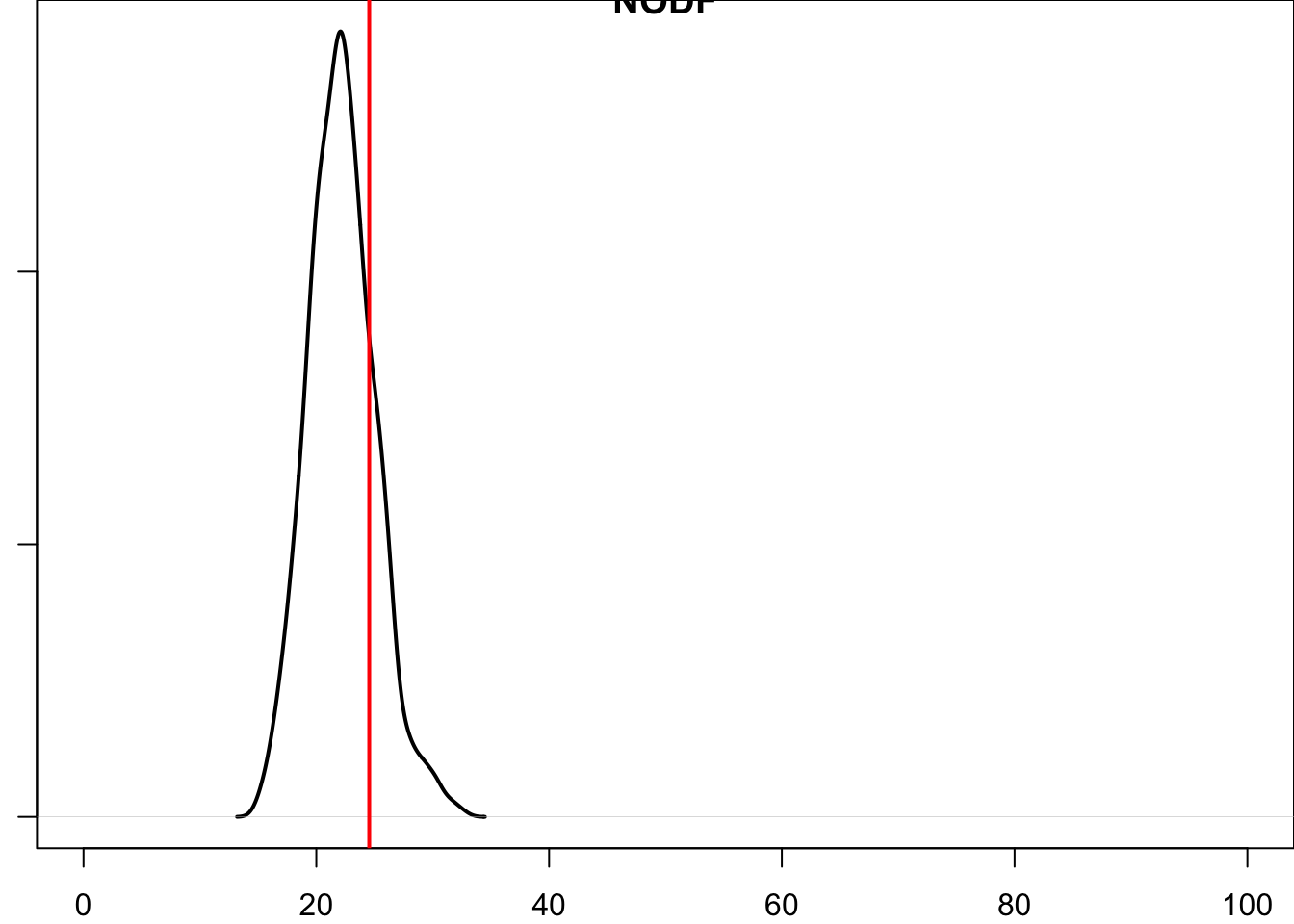
What we see is that the NODF (nestedness) value of the empirical dataset—the red line—sits within the bulk of the null-model NODF distribution (it is a bit above the null mean, but well inside the spread of null values). That is, our empirical value would likely not be considered either more or less nested than chance alone.

Checking results

Before we get to $p$-values, it is always worth checking if the null model we are using actually has the properties that we want. Relative to the empirical network, the swap.web algorithm is supposed to: 1) maintain the connectance; and 2) maintain the row and column sums (the marginal totals). Let’s check that it is actually doing that. We’ll calculate the mean and standard deviation of connectance across all 999 networks; we should be getting an exact or very close to exact match with our empirical connectance, and a standard deviation that is either zero (meaning all of the null networks have the exact same connectance) or very very small. We can then compare the row and column sums.

We’ll start with connectance:

# calculate connectance across the null networks
Cnulls <- sapply(nulls, 
                 function(x){
                   networklevel(x, index = "connectance")[1]
                   })
Cempirical <- networklevel(Safariland, index = "connectance")[1]
SDnulls <- sd(Cnulls)

## mean connectance of null networks = 0.1604938

## connectance of empirical network = 0.1604938

## standard deviation of null networks = 0

Looks great: connectance is exactly the same between the two, and the standard deviation in connectance in the null networks is zero, meaning that each and every null network has the exact same connectance as our empirical network.

Still, it is worth trying this, because sometimes—even in recent versions of bipartite—we have had the experience where these null models do not perform exactly as expected. In those cases, usually if we start a new R session and re-try, it works… but again, it is definitely worth checking.

Now let’s check the marginal totals (the row and column sums). This one is just a little trickier, because there is one value for each species in the network, not just one numeric value for the entire network (as there was with connectance). To account for that, we will put the values—for both the row and the column sums—into a data frame, with rows as species and a column for each of the empirical data and the means of the null models. A nice way to check this formally is then to subtract those two columns; if they are exactly the same (as they should be), then the difference for each value would be zero.

We will do the procedure for both the pollinators and the plants, but we will just display the results in tabular form for the 9 plant species in the “Safariland” dataset to save space.

# calculate row sums across the null networks
Rsums.nulls <- sapply(nulls, 
                      function(x){ rowSums(x) })
# this returns a 9 x 999 matrix, with one column for each null model
# now take the mean across all of those row sums:
Rsums.mean <- apply(
  Rsums.nulls,
  MARGIN = 1,
  FUN = function(x){ mean(x) })

# we'll put this into a data frame along with the empirical row sums:
comper = data.frame(empirical = rowSums(Safariland), 
                    null = Rsums.mean)

# we will check that out in just a second, but first we'll add the col sums:
Csums.nulls <- sapply(nulls, 
                      function(x){ colSums(x)})

Csums.mean <- apply(
  Csums.nulls,
  MARGIN = 1,
  FUN = function(x){ mean(x) })

comper2 = data.frame(empirical = colSums(Safariland),
                     null = Csums.mean)

# bind row & col sum dataframes together:
comper = rbind(comper, comper2)

# subtract null values from empirical values
# (all should be zero if algorithm performing correctly)
comper$difference = comper$empirical - comper$null

# display
kable(comper[1:9, ], row.names = TRUE) %>% 
  kable_styling(
    full_width = FALSE,
    position = "left",
    bootstrap_options = "condensed"
)

	empirical	null
Aristotelia chilensis	790	790
Alstroemeria aurea	208	208
Schinus patagonicus	15	15
Berberis darwinii	72	72
Rosa eglanteria	15	15
Cynanchum diemii	20	20
Ribes magellanicum	5	5
Mutisia decurrens	1	1
Calceolaria crenatiflora	4	4

Looks great—all of the row sums (plant interaction totals) are the same between the null models and the empirical network. Again, the code above included all of the column sums (pollinator interaction totals), as well as a column for difference between empirical row/column sums and mean null model row/col sums. We could easily assess if there were any departures from zero with this line of code: which(comper$difference!=0). If it returns integer(0) you know that they match perfectly (in this case, they do).

Of course, we didn’t check out the standard deviations here, so there is a small chance that there is some variation across the null models (but a pretty tiny chance indeed, given that we see integers for all of the mean values…) but that is something that would be easy to add to the code above if you were interested.

Bringing this back full circle, that means that the swap.web algorithm is doing what we expected relative to the empirical data:

maintaining the same connectance
maintaining the same row and column sums

while we didn’t do an explicit check to see if the total number of interactions is the same between the two, we couldn’t maintain the same row and column sums and also have a different total number of interactions, so we are safe there as well.

p-values

Our first pass at the null model analysis above was graphical. We can formalize this test in a very straightforward way, calculating a $p$-value by assessing the rank of the empirical value relative to the nulls. Let’s imagine a case in which the empirical value was more-nested than almost all of the nulls. If we were to generate 99 nulls, and out of the 100 total networks we were assessing (the 99 nulls + the 1 empirical network), the empirical network was the 5th-most nested (i.e. 4 null models were more nested), then the $p$-value would be exactly 0.05 (5 out of 100). One way of conceptualizing that is that if the empirical value was part of the same distribution as our null models, we could assign it a rank in that distribution at random. And there would only be a 5% chance ($p$ = 0.05) that the rank would be 5th or more extreme (4th, 3rd, 2nd, or 1st).

Similarly, if the empirical network were the most-nested of all, the $p$-value would be 0.01 (1 out of 100). Two lessons from that: first, it makes the $p$-value calculations slightly easier if you generate {some power of 10 minus 1} null models, e.g. 99 or 999 or 9,999 null models. Still, that is not strictly required. And second, the more null models you calculate, the greater the precision you have in your $p$-value. The examples above were for 99 null models; if you were to use 9,999 nulls and your empirical network were the top-ranked one, the $p$-value would be 0.0001 (1 in 10,000). The caveat there is that the more null models you calculate, the longer it takes. Typically if you’re after assessing statistical significance in the traditional sense, you will want to use more than 99 null models, as that is pretty coarse, especially since you can have slight variations in the $p$-value if you re-run your null models. Still, once you get to 999 you should (usually) know if the $p$-value is less than the standard $\alpha$ value of 0.05. If you have a borderline value, you might want to amp up the resolution by running more null models.

It’s also worth noting that the $p$-values as described above are for a one-tailed test. For example, if you had the a priori hypothesis that your empirical network was more nested than you would expect by chance, then you could assess that with a one-tailed test. If you wanted to see if your network was either more or less nested than chance alone, for the example with 99 null models, if your empirical data were either the most or the least nested, there is a 1 in 100 chance of either of those situations happening. So you would need to multiply the $p$-value by 2 to compensate: there is a 2 in 100 chance of either occurring, so the $p$-value for either situation would be not 0.01, but 0.02.

p-value calculation

With all of that in place, we can write code to calculate the (two-tailed) $p$-value. The standard, symmetric way to do this (Davison & Hinkley 1997; Manly 2007) is:

count how many nulls are at least as extreme as the empirical value on the low side, and separately on the high side
add 1 to each count (this counts the empirical value itself, and keeps the smallest possible $p$-value at $1/(N+1)$ rather than 0), and divide by $N + 1$
take the smaller of those two one-tailed $p$-values and double it (two-tailed), capping at 1

Wrapped in a small function:

# two-tailed permutation / null-model p-value
two_tailed_p <- function(nulls, obs) {
  n <- length(nulls)
  p_low  <- (1 + sum(nulls <= obs)) / (n + 1)
  p_high <- (1 + sum(nulls >= obs)) / (n + 1)
  min(1, 2 * min(p_low, p_high))
}

pval <- two_tailed_p(Inulls, Iobs)

## p = 0.352

In this case the $p$-value is 0.352—the Safariland network is not significantly more or less nested than chance under the swap.web null model. (This is the same two_tailed_p() helper used in the 2026 networks exercises.)

Take-home

Together these examples point to a few take-home messages:

the precise null model you use for your analysis matters—different null models can give you completely different results
in general, a good default is to use a more conservative null model algorithm, i.e. one that holds constant more features of the empirical network
- but be careful especially with small networks that your null models are not too constrained to generate substantive enough variation
always check your null models to make sure they are performing as expected
use a two-tailed $p$-value as a default, unless you have laid out an a priori hypothesis that includes directionality (e.g., “I hypothesize that this network will be less-nested than chance alone would predict”)

Exercise 8

Analyze NODF for the “Safariland” dataset using the r2dtable null model,

graphically and
by calculating the (two-tailed) $p$-value. You should get a qualitatively different result relative to using swap.web. Describe where the empirical value falls out relative to the null models.

Bonus exercise

Using the information above on the correlation among network metrics, as well as descriptions of the null models, offer an interpretation as to why the two null models yield qualitatively different results.

Double bonus exercise

Try one of the null models implemented in vegan, in particular quasiswap_count. Here is some code that should help you; the syntax is different for the vegan implementation relative to bipartite and in addition vegan returns the null models not as a list, but instead as a 3-dimensional array. The latter means you need to take a slightly different approach when calculating NODF (or any other metric) across the null models.

## Alternative: use vegan::nullmodel rather than bipartite
# install.packages('vegan', dependencies = TRUE)
library(vegan)
# Require first setting up a null model, then separately simulating it
n.vegan <- vegan::nullmodel(Safariland, "quasiswap_count") #setup
nulls.vegan <- simulate(n.vegan, nsim = 999)               #simulation

# The vegan `simulate` method returns a 3-dimensional numeric array
# so need to modify the code used for the bipartite nulls
# use `apply` rather than `sapply` with MARGIN = 3
Inulls.vegan <- apply(nulls.vegan, 
                      MARGIN = 3, 
                      FUN = function(x){nestednodf(x)$statistic[3]})

If you go for the “double bonus” round, you should get again a qualitatively different result relative to swap.web. This is somewhat curious as the two methods are supposed to be very similar….

Comparing networks

Assessing a single network against a null model has its place, but it is limited. The more common—and usually more interesting—question is whether network metrics differ between two or more empirical networks: drought vs. non-drought years, urban vs. rural sites, along an elevational gradient, and so on.

The obstacle is the one from Relationships among metrics: it is very rare for two empirical networks to share species richness, number of interactions, and sampling effort, and those things strongly drive metric values on their own. So a raw difference in (say) connectance between two networks can easily be an artefact of one being smaller or less-sampled, rather than a real biological difference.

Why not just use $z$-scores?

The long-standing fix was to compute a $z$-score for each empirical metric relative to its own null distribution, and then compare those across datasets. Song, Rohr & Saavedra (2017, Journal of Animal Ecology) showed that the $z$-score itself depends on network size, so this does not fully solve the problem. They proposed a size-corrected alternative, $NODF_c$—but only for nestedness.

Downsampling

A more general approach, which works for any metric: make richness and sampling effort equal across the networks by randomly downsampling the larger or better-sampled network down to the size of the smaller one—many times—to build a distribution. Then compare the smaller network’s observed metric value to that distribution. Any difference that survives is more defensibly biological.

A worked example is Morozumi et al. (2022, Oikos, “Simultaneous niche expansion and contraction in plant–pollinator networks under drought”): three RMBL plant–pollinator networks across two drought and three non-drought years. Drought years had far fewer interactions and lower richness (many plants did not bloom at all), which makes direct metric comparisons unreliable. Diet theory predicts pollinators broaden their floral niches under drought, which would show up as higher connectance—but lower-richness networks have higher connectance by default, so the raw pattern is confounded. Morozumi et al. downsampled the non-drought networks to a comparable number of interactions and/or species as the drought networks, and compared. A useful variant keeps only the species present in both conditions before downsampling, which helps separate “the set of species changed” from “the same species changed their behavior”.

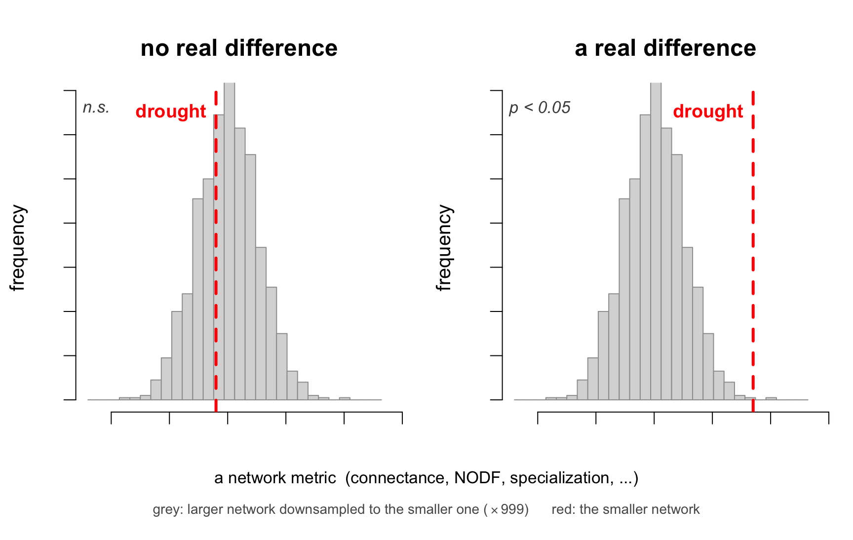
The logic of the comparison, drawn schematically below with made-up data (in the style of Morozumi et al. 2022, Fig. 1): repeatedly downsample the larger (non-drought) network to the size of the smaller (drought) one to build a null distribution (grey), then see where the drought network’s observed metric (red) falls. If it lands inside the distribution the apparent drought effect was an artefact of size; if it falls in the tail, the difference is defensibly biological.

Exercise 2 in the workshop’s networks exercises walks through implementing this on the drought / non-drought RMBL data.

Structure & Stability

Networks are useful descriptors of community structure but also they matter for the stability of communities. Researcher have investigated the effect of networks structure on community dynamics including their stability since Robert May’s pioneer work in 1972 showing mathematically that increased levels of complexity decreases stability of communities. Some concepts of stability you will find in the network literature include:

Local stability: A system is locally stable if it returns to its original state after being slightly disturbed. Mathematically, local stability is often analyzed through the concept of stability analysis, which involves examining the behavior of a system near an equilibrium point. One common method used to analyze local stability is through linearization, where the system’s dynamics are approximated by a linear model around the equilibrium point. This is the concept used by Robert May’s work and because its simplicity, has been used by many in the field. However it has important limitations, including the assumption of a local equilibrium, the inability of evaluating any but small perturbations, and the assumption of linear dynamics at equilibrium.
Resilience: Time to return to a local equilibrium after slightly perturbing the system away from it.
Structural Stability: In local stability analysis the perturbations act on state variables, limiting the analysis to changes in species abundances only. Conversely, one can study other perturbations using structural stability analysis. A system is considered to be structurally stable if any smooth change in the model itself or in the value of its parameters does not change its dynamic behavior (e.g., existence of equilibrium points, limit cycles, chaos, etc).
Feasibility: All the constituent species from the community attain positive abundances at equilibrium.
Species persistence: Typically used in studies of computer simulations, defined as the fraction of initial species that persists until the end of the simulations.
Robustness against species extinctions: Typically defined in studies of computer simulations as the resistance of a network to loose more species (as secondary extinctions) as result of primary extinctions, which are typically simulated as the removal of species from the network.

We will elaborate more on the effect of network structure on network dynamics and stability in day 3.

Session Info

sessionInfo()

## R version 4.6.0 (2026-04-24)
## Platform: aarch64-apple-darwin23
## Running under: macOS Sequoia 15.7.9
## 
## Matrix products: default
## BLAS:   /Library/Frameworks/R.framework/Versions/4.6/Resources/lib/libRblas.0.dylib 
## LAPACK: /Library/Frameworks/R.framework/Versions/4.6/Resources/lib/libRlapack.dylib;  LAPACK version 3.12.1
## 
## locale:
## [1] en_US/en_US/en_US/C/en_US/en_US
## 
## time zone: America/Denver
## tzcode source: internal
## 
## attached base packages:
## [1] stats     graphics  grDevices utils     datasets  methods   base     
## 
## other attached packages:
##  [1] bipartite_2.24        sna_2.8               network_1.20.0       
##  [4] statnet.common_4.13.0 kableExtra_1.4.0      lubridate_1.9.5      
##  [7] forcats_1.0.1         stringr_1.6.0         dplyr_1.2.1          
## [10] purrr_1.2.2           readr_2.2.0           tidyr_1.3.2          
## [13] tibble_3.3.1          ggplot2_4.0.3         tidyverse_2.0.0      
## [16] vegan_2.7-3           permute_0.9-10        knitr_1.51           
## 
## loaded via a namespace (and not attached):
##  [1] dotCall64_1.2      spam_2.11-3        gtable_0.3.6       xfun_0.60         
##  [5] bslib_0.10.0       lattice_0.22-9     tzdb_0.5.0         vctrs_0.7.3       
##  [9] tools_4.6.0        generics_0.1.4     parallel_4.6.0     cluster_2.1.8.2   
## [13] pkgconfig_2.0.3    Matrix_1.7-5       RColorBrewer_1.1-3 S7_0.2.2          
## [17] lifecycle_1.0.5    compiler_4.6.0     farver_2.1.2       fields_17.3       
## [21] textshaping_1.0.5  maps_3.4.3         htmltools_0.5.9    sass_0.4.10       
## [25] yaml_2.3.12        pillar_1.11.1      jquerylib_0.1.4    MASS_7.3-65       
## [29] cachem_1.1.0       nlme_3.1-169       tidyselect_1.2.1   digest_0.6.39     
## [33] stringi_1.8.7      bookdown_0.48      splines_4.6.0      fastmap_1.2.0     
## [37] grid_4.6.0         cli_3.6.6          magrittr_2.0.5     withr_3.0.2       
## [41] scales_1.4.0       timechange_0.4.0   rmarkdown_2.31     igraph_2.3.1      
## [45] otel_0.2.0         blogdown_1.24      hms_1.1.4          coda_0.19-4.1     
## [49] evaluate_1.0.5     viridisLite_0.4.3  mgcv_1.9-4         rlang_1.2.0       
## [53] Rcpp_1.1.1-1.1     glue_1.8.1         xml2_1.5.2         svglite_2.2.2     
## [57] rstudioapi_0.18.0  jsonlite_2.0.0     R6_2.6.1           systemfonts_1.3.2

Last updated on Sep 3, 2026