Dynamics

Dynamics and stability

Motivation

It almost goes without saying, but in order to integrate ecological data and theory one needs to understand the fundamental tools of theoretical ecology. In our context of plant-pollinator interactions, those tools invariably involve the mathematics of “dynamical systems”, including calculus (a little analytic but mostly numerical), a lot of algebra (i.e. moving symbols around), and linear algebra (matrices). The greatest challenges in learning these tools are typically getting used to and practiced in working with symbols translating/implementing the “pen-and-paper” mathematics as computer code. In our experience, both come from simple repeated exposure and practice (and hence motivation and interest). Moreover, just because someone is already comfortable with mathematics does not mean they’re already comfortable with coding (and vice versa).

Overview

Our goal is to introduce you to the foundations of dynamical systems analysis that underlies much of ecological theory. Going back-and-forth between the mathematics and the code, we’ll progress through the analysis and simulation of single-species exponential and logistic growth, to the (graphical) analysis and simulation of two-species mutualistic interactions, to the simulation-based analysis of many-species mutualistic networks. In the process, we’ll touch on concepts and tools including steady states, local (a.k.a. linear) stability analysis, and isoclines.

Throughout, we will use the symbol $N$ to represent population size, as it does in nearly all population models in ecology.

Required R-packages

We’ll need the deSolve package to integrate our differential equations with respect to time.

# install.packages('deSolve', dependencies = TRUE) # use to install if needed
library(deSolve)

Exercise code

In addition to the in-text links below, you can download what you’ll need in this GoogleFolder.

Exponential growth

For a start preceding the introduction of exponential growth, see the Of Potential Interest page.

We will take as our starting point the differential equation,

$$ \frac{dN}{dt} = rN . $$ The left-hand-side of this equation is little more than a tangent slope: the change in population size given a change in time (i.e. how much the population size changes over a small amount of time).

The right-hand side is a product of the population size $N$ (at any given instant in time) and $r$ is the intrinsic per capita growth rate. The intrinsic growth rate is nothing more than the difference between the rate at which the average individual gives birth, $b$, and the rate at which the average individual die, $d$. Together, they left and right-hand sizes of the equation represent the model of exponential growth.

The key to the exponential model is that the per capita birth and death rates (and thus $r$) are themselves independent of $N$. As a result, the population will growth if $r$ is net positive ($b > d$) and will exhibit exponential growth. Conversely, the population will shrink if $r$ is net negative ($b < d$) and will exhibit exponential decay.

Projections

To use the differential equation $\frac{dN}{dt}=rN$ to project population sizes into the future we need to integrate the differential equation. Integrating from time $0$ to some time $T$ in the future, and assuming an initial population size at time zero of $N_0$, we get:

$$ \int_0^T \frac{dN}{dt} dt = \int_0^T r N dt \implies N_T = N_0e^{rT}, $$ where $e$ is Euler’s number aka the base of the natural logarithm, which rounded to 5 digits is: 2.71828. (Think of Euler’s number $e$ as the anti-logarithm $ln$ or $log_e$, just like $2^x$ is the anti-logarithm of $log_2$.) Euler’s number is deeply rooted to multiplicative (exponential) processes.
The fact that an exponential shows up in the equation is why the modelis referred to as the model of exponential growth.

Integration

Analytically integrating $\frac{dN}{dt}$ to obtain a projection equation for the exponential model is relatively straightforward. Doing so is also possible for other models, such as the Logistic model that we will look at next. However, for most population dynamic models in ecology (especially multi-species models), analytical integration isn’t possible. So what we want to do is to develop a platform for modeling population dynamics that allows us to numerically solve integration problems (i.e. solve with calculations done by the computer rather than analytically), in a way that is extensible to much more complex problems. And to learn such approaches, it is definitely best to start with a simple model—and the extremely simple exponential growth model is perfect for this.

The tool we will work with is the ode() function of the deSolve package. deSolve implements multiple different numerical methods for solving ODEs (ordinary differential equations), which are the kinds of equations we will be working with in this workshop (equations that have $\frac{dN}{dt}$ on the left-hand side). The deSolve package is very powerful and allows us to numerically solve even very complex multi-species network models (which we will be working up to throughout the day). But that flexibility means that it has a complex structure, which can admittedly be somewhat confusing when you are first starting to use it.

The function ode() requires a minimum of four input arguments, ode(y, times, func, parms):

y is initial starting size of the variable (i.e. $N(0)$)
times are the vector of time points $t$ at which we want ode to spit out the values of $N(t)$
- e.g., times = 1:100 or times = seq(from = 1, to = 200, by = 0.2)
func is our ODE model for $dN/dt$ (written as a function with its own arguments)
parms is a vector of the ODE model’s named parameters

The argument func (i.e. our ODE model) that we provide ode must be defined in a particular way that may feel a little redundant with the input that we pass to the ode function because they have to be working in parallel. The arguments that the function must have are (in order): (1) times; (2) the variable(s)—here, population size; and (3) the parameters used in our model.

In our code below, we will also take advantage of a facet of R that is not very well known. You can create a vector in R where you name the elements, for example my.vector = c(marmot = 3.2, pika = 47.6, ground.squirrel = 18.4). With a named vector, you can then access the elements via their name indicated with quotation marks: for the example above if you entered my.vector['pika'] you would get back 47.6. We can use that with our parameters to clearly name which parameter is which. Here we really just have one parameter (r) and one response / output variable (N), but still, it is useful to name them parameters <- c(r = 0.2).

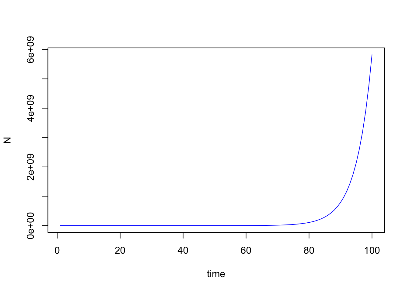
Let’s try it

We’ll use the exact same setup in terms of values of $r$ and $N(0)$ as we did in the plot above.

# library(deSolve)

# set initial conditions of response variable
popn <- c(N = 12)

# Parameters
parameters <- c(r = 0.2)

# Time sequence
times <- seq(0, 100, by = 1)

# "exp.model" stands for "exponential growth model" 
exp.model <- function(time, popn, parameters) {
    # exponential growth model, dNdt = r*N:
    dNdt <- parameters['r'] * popn['N']
        # the function must return a list (even if it is just one element):
    return(list(dNdt))
  }

# Solve the ODE
out <- ode(y = popn, times = times, func = exp.model, parms = parameters)

# Plot the output
plot(out, ylab = "population size, N", col = "blue")

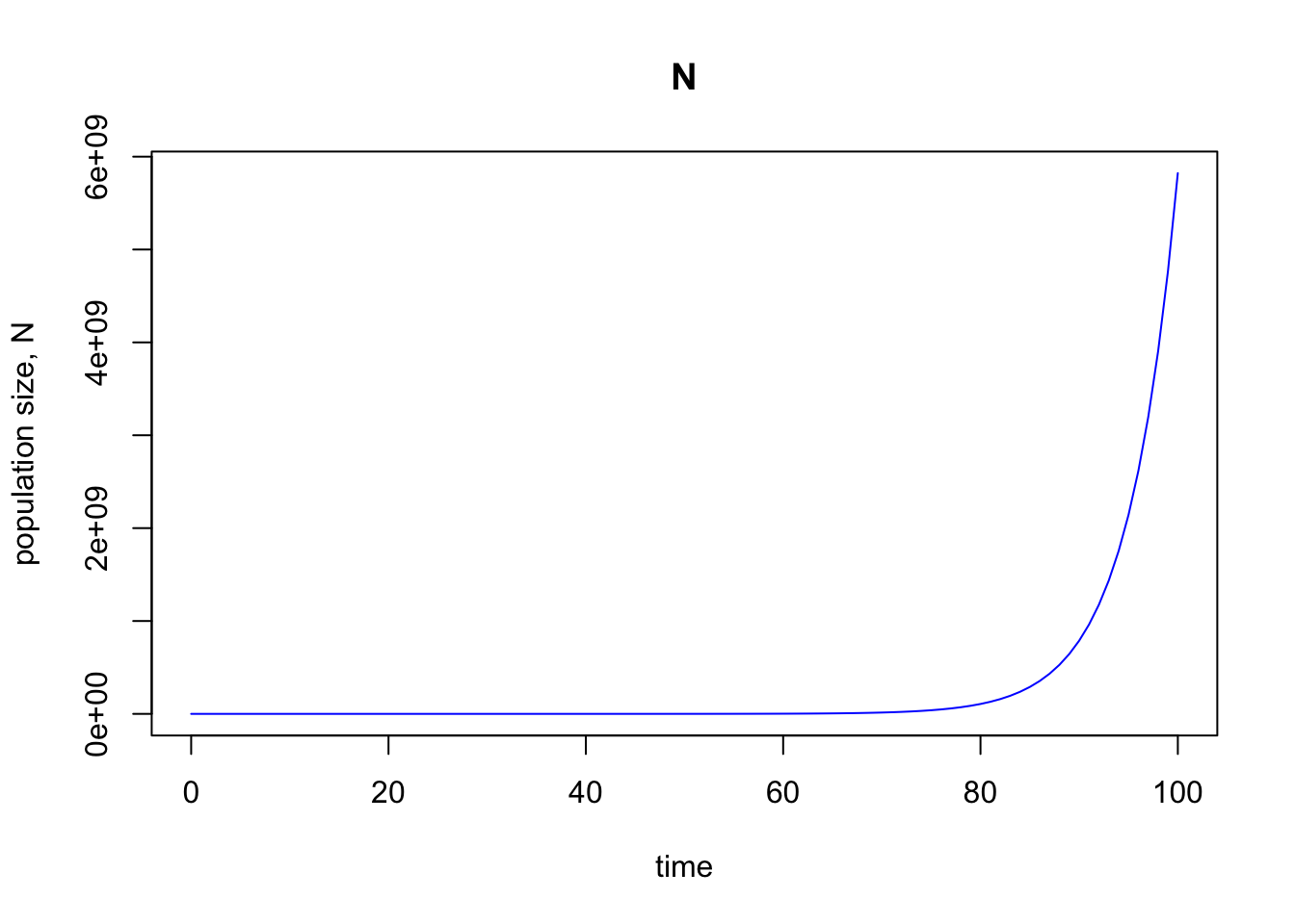
Great—this looks identical to our previous plot, which is what we wanted. If you view it with View(out) you can see that there are two columns in the output from ode, one for time and one for population size.

Exercise 1

Alter the code above to run a simulation of exponential growth over 200 time steps, for a population with an initial size of 202 individuals and $r$ = 0.225.

Logistic growth

As discussed above, the exponential growth model approximates reality by assuming that per-capita birth and death rates are constant—an individual has a set number of offspring and a fixed chance of dying over a given time period. If you are competing with lots and lots of conspecifics to get enough food, or you’re under heightened risk of disease, it’s likely that your chance of dying in a given time will go up, and that the number of offpsring you produce will go down. There are many different empirical datasets from around the world and a range of different kinds of organisms (plants, animals, microbes, etc.) showing this pattern of negative density-dependence—in other words, $r$ is not a constant with respect to population size, but instead changes as a function of population size.

To model density-dependent growth, we’ll start from the exponential growth equation, which again, is:

$$ \frac{dN}{dt} = rN . $$

If we divide both sides by $N$, we get

$$ \frac{1}{N}\frac{dN}{dt} = r . $$

The left-hand side $\left( \frac{1}{N}\frac{dN}{dt} \right)$ we have the term for per-capita population growth rate, and on the right hand side we have $r$ (which we are again here defining as a constant). This equation may strike you as almost tautological, since we defined $r$ as the per-capita population growth rate, but perhaps another way to think of it is that it is reassuring that re-arranging the equation brings us back to our definitional equalities.

The point here is that we have re-arranged things to have the per-capita population growth rate on the left (as the response variable), and a constant on the right. Now we can change the right-hand side from a constant to some function of population size to reflect density dependence.

One of the simplest ways to incorporate density dependence is to assume that $\left( \frac{1}{N}\frac{dN}{dt} \right)$ is a linear function of density; this ultimately yields the logistic growth equation.

In formulating linear density dependence, the hypothetical maximum possible per-capita population growth rate occurs when the population is approaching zero (i.e., no possible density effects); obviously that value would never be realized if the population were actually zero, so think about $\left( \frac{1}{N}\frac{dN}{dt} \right)$ as approaching $r$ as $N$ tends towards 0. A line with a negative slope (decreasing function of $N$) would at some point then cross the $N$-axis, at which point the per-capita population growth rate would be zero; and would keep going down as the population size increases (at which point the per-capita populationgrowth rate would be negative).

Here is what such a linear formulation would look like:

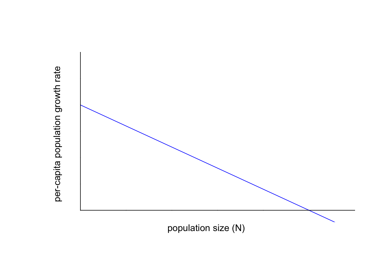
Next, we will re-define $\left( \frac{1}{N}\frac{dN}{dt} \right)$. In our formulation of the exponential growth model, $r$ was the constant or fixed per-capita population growth rate. Now, we will set $r$ to be the (intrinsic) maximum population growth rate in the absence of competition. In other words, $r$ is the y-intercept of the graph above.

We can also define the $N$-intercept of the line. Population biologists call the $N$-intercept the carrying capacity, $K$. At the carrying capacity, then, is where the population stops changing in population size, since the per-capita population growth rate is (net) zero. Births and deaths are still happening, but they cancel each other out; all deaths are replaced by an equal number of births.

Let’s add those labels to our plot:

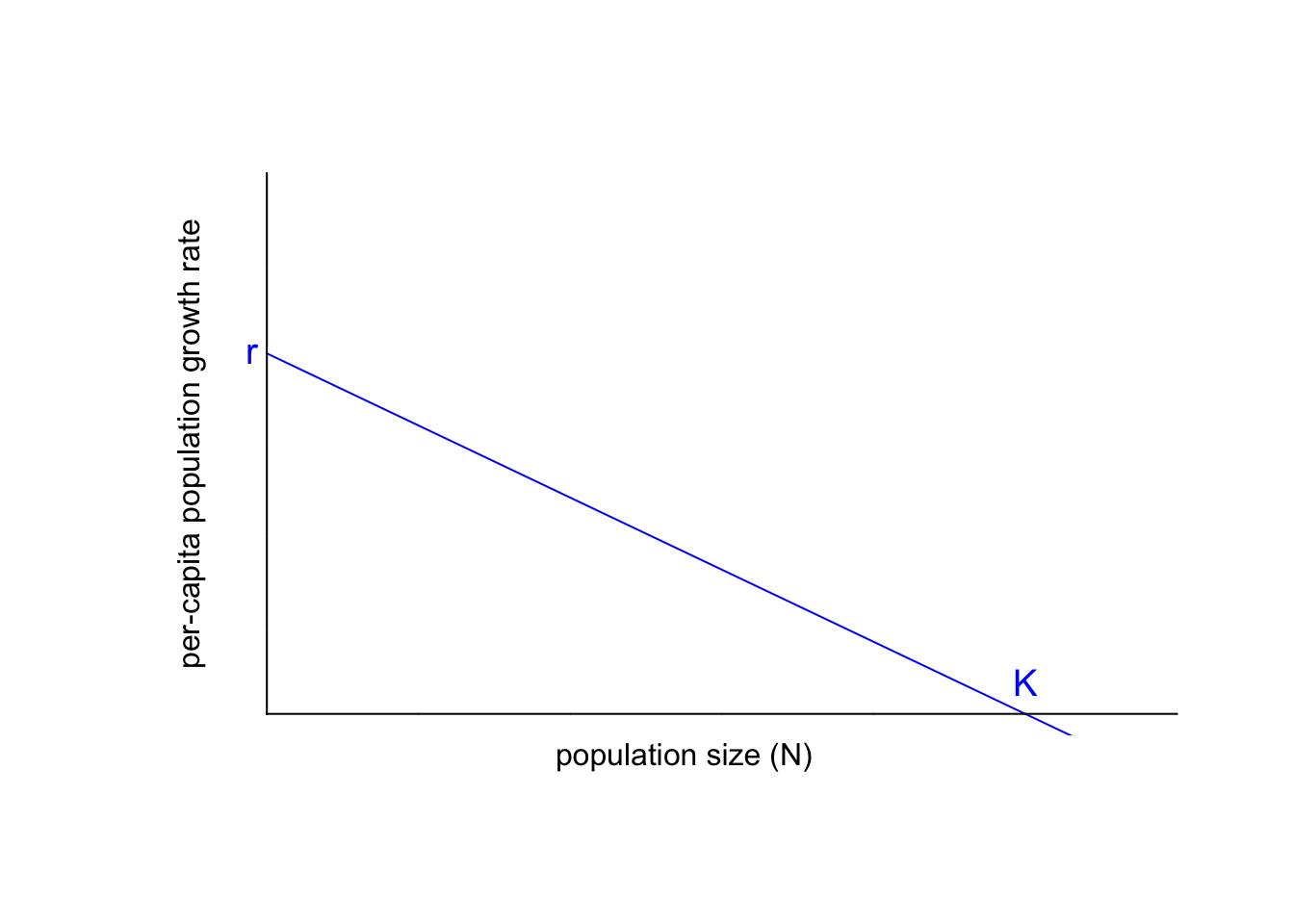
With those definitions in mind, let’s get back to our task of setting the per-capita population growth rate $\frac{dN}{dt}\frac{1}{N}$ to the linear function above, using the generic formula for a line of $y = m x + b$:

$$ \frac{1}{N}\frac{dN}{dt} = r - \frac{r}{K} N, $$ where we have replaced $x \rightarrow N$, $b \rightarrow r$ is the intercept, and $m \rightarrow -\tfrac{r}{K}$ is the slope. The slope ($m$), is defined as “rise” (change in the y-axis) over “run” (change in the x-axis). As the population moves on the x-axis from 0 to $K$, the per capita growth rate changes from $r$ to 0. Thus, the “rise” is $-r$ and the “run” is $K$, so $m = \frac{-r}{K}$.

Rearranging by factoring out $r$, we have $$ \frac{dN}{dt}\frac{1}{N} = r\left(1 - \frac{N}{K}\right) $$ and thus, reverting to thinking about the population growth rate, we have $$ \frac{dN}{dt} = rN\left(1 - \frac{N}{K}\right) . $$

This is the logistic growth equation that is ubiquitous in population ecology.

We’ll model logistic growth using deSolve as we did above for exponential growth. We actually don’t have to change very much; the time part is the same and we still keeping track of just one population. We’ll need to change the formulation of the model itself, of course, and add parameter $K$ to the parameter vector.

# library(deSolve)

# set initial conditions of response variable
popn <- c(N = 12)

# Parameters
# only change from exponential is adding `K`
params <- c(r = 0.2, 
            K = 250000)

# Time sequence
times <- seq(0, 100, by = 1)

# function for ode
logistic.model <- function(time, popn, parameters) {
    # logistic growth equation:
    dNdt <- params['r'] * popn['N'] * (1 - popn['N'] / params['K'])
    return(list(dNdt))
  }

# Solve the ODE
out <- ode(y = popn, 
           times = times, 
           func = logistic.model, 
           parms = params)

# Plot the output
plot(out, 
     ylab = "population size, N", 
     col = "blue")

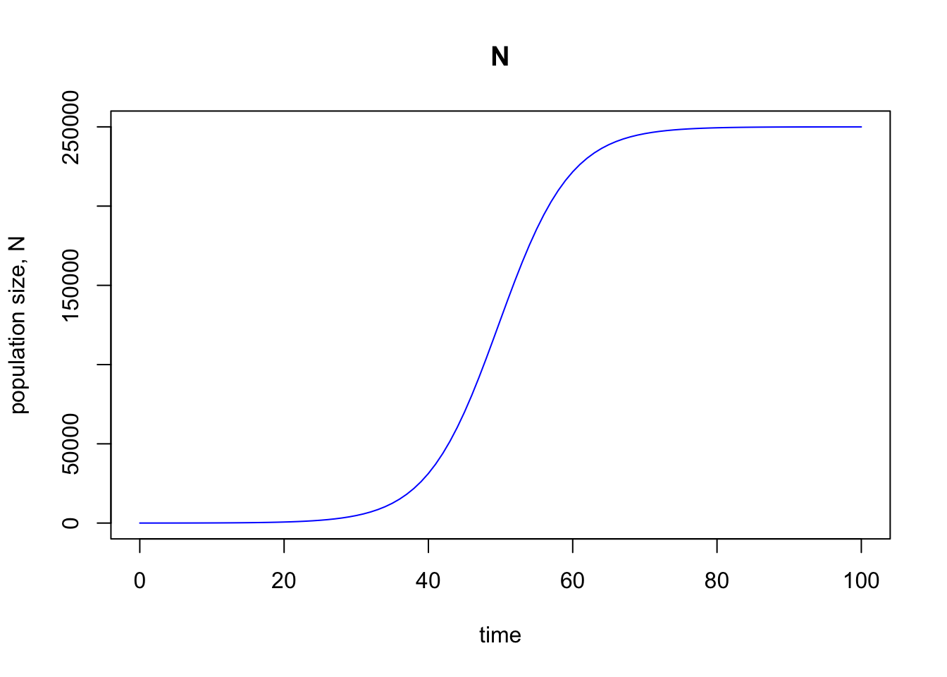
Again, looks good—we see what we expect, which is that the population grows exponentially initially, but as the population increases, that growth slows down until it plateaus out at the steady state value of $K = 250,000$.

Compact code

For the code above, we have just three input values that need specifying: the population size $N$ (a variable), and two fixed parameters: the (maximum) per-capita population growth rate $r$ and the carrying capacity $K$. The code above refers to different places where we could find those input values (separating the variable from the parameters), and it works well enough.

But we can make the coding a little easier on ourselves—and perhaps more importantly, more transparent and scalable—with just a little bit of additional code “magic”. The code chunk below does the same thing as the code above, but the code for the model itself is much more compact and streamlined, using the variable / parameter names themselves (e.g., r) rather than having to reference the name of the object in which to look for those (e.g. params['r']).

Again, for exponential or logistic growth, it isn’t a very big deal to have to include the name of an object like params, but as our models become more complicated, it makes our life much easier to just include the name of the variables. We can do that with the addition of just a single line of code:

with(as.list(c(popn, params)), {...})

This line of code allows us to directly use the names of the variables and parameters in the objects (popn and params) that we included in that argument—and we could pass along as many objects as we wanted, making sure that the values within them are named, e.g. params <- c(r = 0.2, K = 250000), but not params <- c(0.2, 250000).

To break down that line of code function-by-function:

c() combines the two vectors (popn and params) into a single vector (you could include as many vectors here as you would like)
as.list turns that vector into a list (which is what the next argument, with requires)
with is the real “magic”: it creates an environment from that list, within which R looks for named values

The ellipses ({...}) in the curly braces in the line of code above signal that we have to include the code for model itself inside the arguments to with() and specifically within the curly braces—see below for how that is done, usually across multiple lines of code.

Let’s take a look at how that is actually implemented. The key difference between the code chunk below and the one above is that we can now specify our model much more directly, compactly, and readably: dNdt <- r*N*(1 - N/K) rather than dNdt <- params['r'] * popn['N'] * (1 - popn['N'] / params['K']):

# library(deSolve)

# set initial condition (at time zero) of our response variable
popn <- c(N = 12)

# Parameters
params <- c(r = 0.2, 
            K = 250000)

# Time sequence
times <- seq(0, 100, by = 1)

# specify the model
logistic.model <- function(time, popn, parameters) {
    # `with` line tells code where to find the named elements in the model
    with(as.list(c(popn, params)), {
    # logistic growth equation--very transparent!:
    dNdt <- r*N*(1 - N/K)
    # again, for `ode` need to return a list, even if it's just a vector
    return(list(dNdt))
    })
  }

# Solve the ODE
out <- ode(y = popn, 
           times = times, 
           func = logistic.model, 
           parms = params)

# Plot the output
plot(out, 
     ylab = "population size, N", 
     col = "blue")

As hoped, we get back exactly the same graph as with our prior code.

Exercise 2

Run the logistic growth code above, and then re-run it with a much larger value of $r$ of your choice, but less than $r = 2$ (keep $K$ the same). Re-name the variable out when you re-run it so you have access to the data from both runs. Plot both curves on the same graph, with two different colors.

To plot the new curve on the same graph, if you called your re-run variable out2, in the line after calling plot, add: lines(out2, col = "green")

Stability

Steady states

The steady-state abundance for a differential equation $f(N)=\frac{dN}{dt}$ is the value $N^{*}$ where $f(N^{*})=0$ (i.e. the special population size $N^{*}$ where the population growth rate is zero). Births and deaths are still happening, but they cancel each other out; the system is at equilibrium.

For the logistic model, there are two possible steady states (i.e. two ways to have $\frac{dN}{dt}=0$): The (ecologically) trivial equilibrium, $N^{*}=0$, and the non-trivial equilibrium, $N^{*}=K$. The first of these is discernible by recognizing that everything in $f(N)$ is multiplied by $N$. The second is solved for with some algebra:

Step 1: Set $$ f(N)=\frac{dN}{dt}=0 $$ Step 2: Solve for $N^{*}$: $$ \frac{dN}{dt}=rN\left(1-\frac{N}{K}\right)=0 $$ $$ rN-\frac{rN^2}{K}=0 $$ $$ r =\frac{rN^2}{K} $$ $$ N =\frac{N^2}{K} $$ $$ NK =N^2 $$ $$ N^{*}=K $$

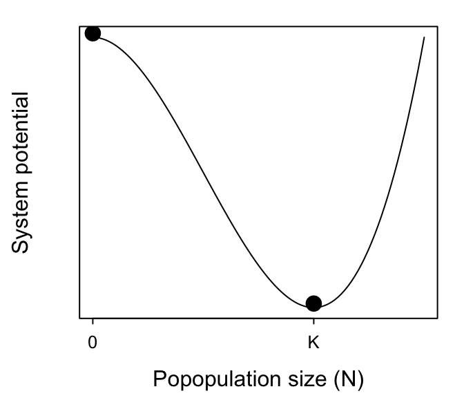
Ball & cup

Through simulation, we found $N^{*}=K$ to be a “stable” in that $\underset{t \to \infty}\lim N(t) = K$ for any initial value $N$ except $N(0) = 0$. Indeed, we found $N^{*}=0$ to be “unstable”; even an infinitesimally small value of $N(0)>0$ eventually got us to $K$, with larger values of $r$ getting us there faster.

To aid intuition, we can describe the driving force behind these dynamics by a landscape¹, with possible population sizes along the x-axis and the steepness of the landscape reflecting corresponding values of $\frac{dN}{dt}$. A ball rolling around this landscape represents any given population size. Gravity causes the ball to roll fast when the landscape is steep (i.e. when $r$ is large), but the ball will slow down the closer it gets to $N^{*}$. The equilibrium $N^{*}=0$ is at the top of an inverted bowl, so any push (any pulse perturbation) to it will cause the population size to roll away from 0. Conversely, $N^{*}= K$ is at the bottom of a bowl, so populations that are perturbed away from $K$ will simply roll back to $K$. Intuitively, the steeper the landscape, the faster the dynamics will be (i.e. the faster the population will return to $K$).

We can evaluate these claims formally. First, by the definition of “asymptotic stability”, an equilibrium $N^{*}$ will be stable to a sufficiently small pulse perturbation if $$ \lambda = \frac{df(N^{*})}{dN} < 0 . $$ Recall that $f(N) = dN/dt$ and that for the logistic we have $dN/dt = r N (1- N/K)$. Therefore we have $$ \lambda = \frac{d}{dN}\left(rN-\frac{rN^2}{K}\right) =r-\frac{2r N}{K} = r- \frac{2r K}{K} = r-2r = -r . $$ This shows that $\lambda$ will be negative for any value $N^{*}>0$ as long as $r > 0$. It thereby confirms our intuition that $K$ is a stable equilibrium. It also confirms our intuition that larger values of $r$ confer greater resilience to the population; it will bounce back from perturbations faster the higher its intrinstic growth rate.

To preview where we’re heading, note that $-r$ is the eigenvalue ($\lambda$) of $f(N^{*}=K)$.²

Analysis

Why is it that $\lambda$ (i.e. the derivative of $dN/dt$ with respect to $N$ evaluated at $N^{*}$) tells us about the stability of $N^{*}$?

To understand this, let’s consider not how our population size $N$ changes in response to a small pulse perturbation but rather what happens to the size of the perturbation itself. This will prove to be a subtle yet useful change in perspective. If $N^{*}$ is indeed stable, then the size of the perturbation $x$ should shrink to zero.

We can think of the size of the population immediately after the perturbation to be $$ N(t) = N^{*} + x $$ The rate of change of that population will be $$ \frac{d N(t)}{dt} = \frac{d (N^{*} + x)}{dt} = f(N^{*} + x) $$ Because $N^{*}$ is a constant with respect to time $t$, it follows that the rate of change of the perturbation is the same. That is, $$ \frac{d x(t)}{dt} = \frac{d N(t)}{dt} = f(N^{*}+x) $$

Now that doesn’t seem to have gotten us anywhere given that $f(N^{*} + x)$ could be a super complicated function. However, regardless of how complicated $f(N^{*} + x)$ is, we can always approximate it! We do so by using a Taylor expansion of $f(N^{*} + x)$ around $N^{*}$. (See Of Potential Utility or Interest page.) That is, $$ f(N^{*} + x) = f(N^{*}) + \frac{d f(N^{*})}{dN} \cdot x + \frac{d^2 f(N^{*})}{dN^2} \cdot \frac{x^2}{2!} + + \frac{d^3 f(N^{*})}{dN^3} \cdot \frac{x^3}{3!} + \dots $$ Notice two things:

By definition, $f(N^{*})=0$, so the first term drops away.
If $x$ is sufficiently small (i.e. $x « 1$), then the 3rd, 4th, etc. terms are vanishingly small.³

Therefore, $$ f(N^{*} + x) \approx \frac{d f(N^{*})}{dN} \cdot x $$ which is equivalent to writing $$ \frac{d x(t)}{dt} \approx \lambda \cdot x $$ In other words, so long as the original perturbation $x$ is small enough, the dynamics of the perturbation will be well-approximated as a simple exponential process! If $\lambda < 0$, then the perturbation will exhibit exponential decay towards 0 over time and thus $N^{*}$ will be stable. If $\lambda > 0$, then the perturbation will exhibit exponential growth and thus $N^{*}$ will be unstable. And if $\lambda = 0$, then the perturbation will not change in size; $N^{*}$ will then be neutrally stable. Our change in perspective to following the size of the perturbation, rather than the population itself, allowed us to do this.

LV Mutualism

Next, we’ll extend our single-species model of logistic growth to consider two interacting species.

The Lotka-Volterra model for mutualism represents two species positively affecting the population growth rate of each other. The model assumes that the population of the two species ($N_1$ and $N_2$) grows logistically and that the interaction benefits received by the populations increases linearly with increasing population size of their mutualistic partner, which is encoded in the following equations:

$$ \frac{dN_1}{dt}=r_1N_1\left(\frac{K_1-N_1+\alpha_{12}N_2}{K_1}\right) \ \frac{dN_2}{dt}=r_2N_2\left(\frac{K_2-N_2+\alpha_{21}N_1}{K_2}\right) $$

The parameters $\alpha_{12}$ and $\alpha_{21}$ are coefficients representing the strength of mutualism. Note that if we set them to zero (i.e. $\alpha_{12} = \alpha_{21} = 0$) we recover the logistic model for each species.

Exercise 3

Let’s focus just on the equation for species 1: $$ \frac{dN_1}{dt} = r_1N_1\left(\frac{K_1-N_1+\alpha_{12}N_2}{K_1}\right) . $$ Assume that $r_1$=0.2$\frac{1}{day}$, $\alpha_{12}$=0.5$[dimensionless]$, and $K_1$=30$\frac{indiv}{m^{2}}$. Let’s also assume that species $N_1$ is at a density above it’s carrying capacity: $N_1=35$$\frac{indiv}{m^{2}}$. Now plug in two different values for the density of species 2: $N_2$=14$\frac{indiv}{m^{2}}$ and $N_2$=8$\frac{indiv}{m^{2}}$. For each of these two values, solve the entire equation for the instantaneous rate of change of the population: $\frac{dN_1}{dt}$. Is the population increasing or decreasing? Reflect on the two outcomes, keeping in mind that species 1 was over its carrying capacity the whole time. Do you see how this equation captures the effects of mutualism? Make sure to track units when plugging numbers! Units help you to better understand models and closely track your calculations.

Exercise 4

Based on your calculations, reflect on how the relationship between $N$ and the carrying capacity, $K$, is affected by the population density of the mutualist species and the strength of the mutualism coefficients, $\alpha_{ij}$. In your thinking, consider how this model captures the effects of mutualism on the fundamental niche.

Isoclines

Now we will develop a graphical understanding of the behavior of the Lotka-Volterra model for mutualism by analyzing their isoclines. Isoclines help us define when the two populations are neither growing nor declining. The combination of densities of species 1 and species 2 that results in a zero per-capita growth rate for species 1 can be found by setting $\frac{dN_1}{dt}=0$ and solving for $N_1$ and $N_2$. The same can be done for species 2 by setting $\frac{dN_2}{dt}=0$ and solving for $N_1$ and $N_2$.

Exercise 5

Solve for the species 1 isoclines by setting $\frac{dN_1}{dt}=0$. Remember to consider both trivial and non-trivial steady states

Exercise 6

Solve for the species 2 isoclines by setting $\frac{dN_2}{dt}=0$. Remember to consider both trivial and non-trivial steady states

Exercise 7

By now you have solved for the species 1 and species 2 isoclines individually. You should have 4 expressions in total: two describing the species 1 equilibrium (one trivial and one non-trivial) and two describing the species 2 equilibrium (one trivial and one non-trivial). Work in groups to plot the 4 isoclines - you may use a piece of paper or the whiteboard. Note that for consistency with my slides, the y-axis should represent species 1’s density ($N_1$ ) and the x-axis should represent species 2’s density ($N_2$), as follows:

Exercise 8

Revisit the different definitions of stability provided at the end of day 1. Identify which of those definitions are appropriate for characterizing the stability of the L-V model of mutualism.

Parameter effects

Much of ecological theory can be derived by understanding how the isoclines of our mathematical models change with changes in parameter values or functional forms, affecting the dynamical outputs of the model. Increasing or decreasing parameter values can represent biological processes of interest, so the effect of those changes on the model isoclines can provide insights on how those processes may affect the dynamics of the study system. We will now understand the ecological theory we obtain from the Lotka-Volterra model of mutualism, which introduces dynamic behavior of mutualisms that are common to many models of mutualism and helps us understand the dynamic implications of important attributes such as mutualism strength and whether the interaction is facultative or obligate to each mutualistic partner.

Understanding $\alpha_{12}$ and $\alpha_{21}$ and mutualism strength

The strength of mutualism can vary as you shift $\alpha_{12}$ and $\alpha_{21}$ with higher values representing stronger mutualism.

Exercise 9

Discuss with your group how you expect the strength of mutualism to affect the coexistence between species. The stability of such coexistence? Do you expect that strong or weak mutualism will allow the persistence of both species?

Now, we will explore isoclines under different parameter values by first loading the code that contains the model. If you looking this in the website, you will need first to open and download the following R code. On Mac, you can just right-click on the hyperlink. On Windows, you will need to open, copy all, and then save as R code:

Two-species Lotka-Volterra mutualism model

In class, we will work off a Rmarkdown file. In it, we will source the above script in order to use the following functions.

Exercise 10

Test your hypothesis using the lvMutualismInteractive() function. Copy and paste the code chunk below in the R console to fix all parameters except $\alpha_{12}$ and $\alpha_{21}$, which you can manipulate.

lvMutualismInteractive(N1_0=10, r1=10.0, K1=100, N2_0=10, r2=10.0, K2=75)

This will create an interactive plot where you can manipulate parameters. Just click on the gear icon on the left-top corner and the manipulator will appear. By default, the plot that is produced shows the abundance of species 1 and 2 over time. However, you can also visualize what’s called a “phase diagram” by choosing “Phase Space” from the drop-down menu at the top of the interactive panel. While “abundance over time” plots $N_1$ and $N_2$ against $t$, the “Phase Space” setting plots $N_1$ against $N_2$. In this plot, the magenta ‘X’ represents the starting point of the trajectory and the magenta triangle represents the ending point of the same trajectory shown in the timeseries. The plot also shows you the location of the $N_1$ and $N_2$ isoclines, the lines where $dN_1/dt$ and $dN_2/dt$ are zero, respectively, which you already solved for.

Tip: Run the model with the following $(\alpha_{12},\alpha_{21})$ pairs: $(0.2,0.3)$, $(0.7, 0.6)$, and $(1, 1.2)$. How does interaction strength affect stability across this range of values?

Note: if you see a warning in the R Console about DLSODA, do not worry, this is expected with the extreme dynamics observed at high alpha values.

Obligate vs Facultative

Up until this point, we have only modeled facultative mutualism where species can enjoy mutualistic benefits to grow more than their carrying capacity, but do not rely on them. other words, in the absence of a mutualist partner, all populations have been able to equilibrate to a positive carrying capacity. The Lotka-Volterra model for mutualism also allows us to model obligate mutualism, where populations require the benefits of mutualism to maintain their abundances above zero. We can obtain obligate mutualism in the model by making the carrying capacities $K_1$ or $K_2$ negative. A negative carrying capacity means that population trajectories will continuously be drawn towards zero, unless the benefits provided by mutualist partners are sufficient to maintain positive abundance.

Exercise 11

Discuss with your group how you expect facultative vs obligate mutualism will affect the stable coexistence (i.e. persistence of both species at plausible abundances) of the model. Which do you think is more likely to facilitate stable coexistence? Draw the isoclines for each case.

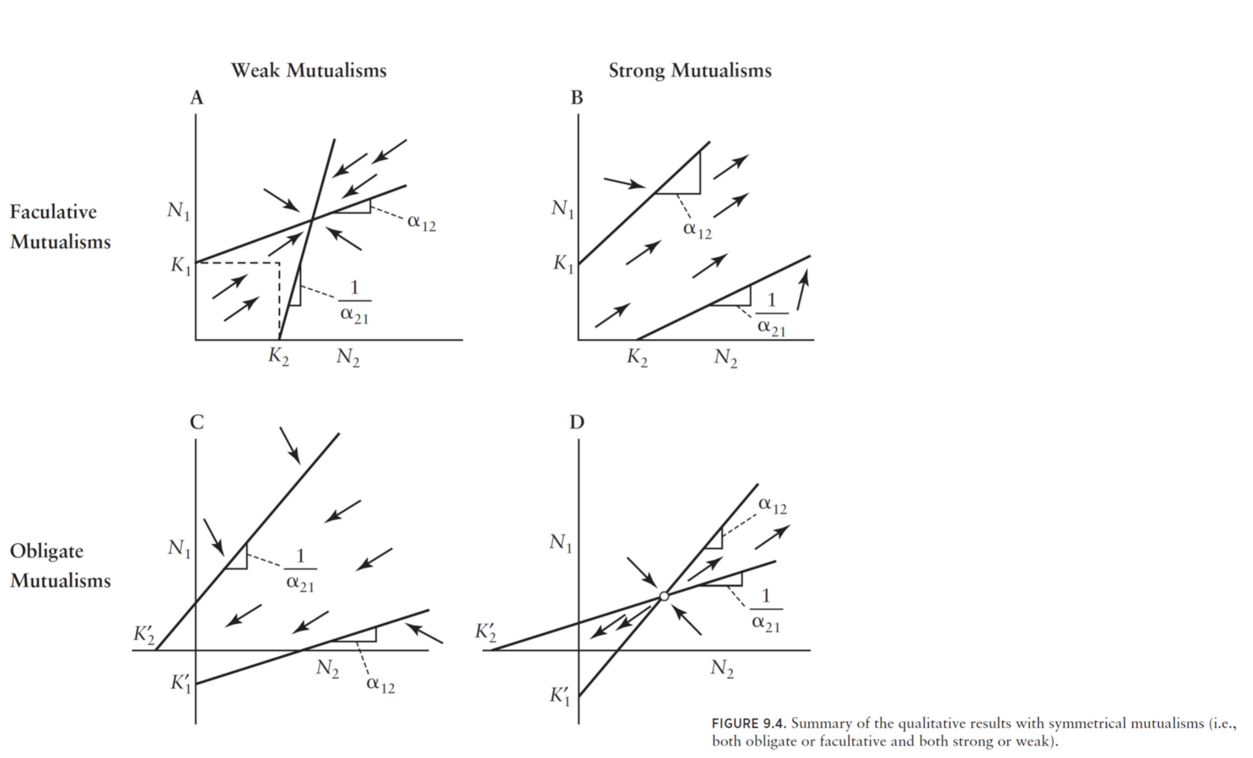
Exercise 12

Reflect as a group on the overarching conclusions about the effect of strong/weak and obligate/facultative mutualism have on stable coexistence, based on the summary figure:

Saturating benefits

Recall that in the L-V model above, the benefit received by each mutualist from their interaction increases linearly with the abundance of their mutualistic partner. This linear benefit causes the positive feedback loop that drives the abundance of the populations to infinity. However, we know that mutualistic benefits do not grow forever but they rather saturate (e.g., fixed number of ovules per plant, consumption saturation just like in other consumer-resource interactions, etc.). We can model that saturation for example by using a Holling type II functional response, which replaces the linear type I functional response exhibited by the model we have used so far, see equations above.

Exercise 13

Sketch a diagram approximating how isoclines of the L-V model might change with saturation of benefit accrual between both mutualists.

Multi-species

The code you downloaded above contains the Lotka-Volterra model of mutualism:

dNdtFunc = function(t, states, param)
    {
        with(as.list(c(states, param)), 
        {
            dN1dt = r1 * N1 * ((K1-N1+alpha12*N2) / K1)
            dN2dt = r2 * N2 * ((K2-N2+alpha21*N1) / K2)
            list(c(dN1dt, dN2dt))
        })
    }

You can see that the equations are written for each species, and that the effect of each species interaction is written as a term indicating the effect of each species on its mutualistic partner. For example, the effect of species 2 on the population growth rate of species 1 is $\alpha_{12} N_2$ (written in the code as alpha12 * N2) on the right side of the equation for $dN1/dt$ (written in the code as dN1dt). Imagine how many lines of code and terms per equation you would need for a networks of, for example, 50 species of plants and 100 species of pollinators. You would need 150 equations (and lines of code) and as many terms per equation as the number of interactions each of those 150 species has, determined by the network. That is clearly not an efficient way to code and think about the problem, plus an error-prone approach when writing manually each interaction per each equation.

A much more efficient approach is thinking in matrices (which encode the networks of species interactions) and connect those matrices to the summation notation in equations. To take this next step, we will use the Lotka-Volterra model of mutualistic networks used by Bascompte et al 2006 (Science, Vol 312, pp. 431-433). This model is simply an extension of the L-V model we used above with linear functional responses, with the only difference that the intra-specific competition encoded in the $(1-N_1/K_1)$ is now represented as self-limitation. There are also minor differences in notation, with subscripts P and A, indicating that a variable or parameter corresponds to that of a plant or animal, respectively. The equations of this network model are: $$ \frac{dN_i^P}{N_i^Pdt} = r_i^P - s_i^P N_i^P + \sum_{j=1}^{n} \alpha_{ij}^A N_j^A $$

$$ \frac{dN_j^A}{N_j^Adt} = r_j^A - s_j^A N_j^A + \sum_{i=1}^{m} \alpha_{ji}^P N_i^P $$ Note that these equations are written for per-capita growth rate but you can recover the population growth rate by multiplying both sides of the equation by the corresponding population size (i.e., $N_i^P$ or $N_j^A$) as $$ \frac{dN_i^P}{dt} = r_i^P N_i^P - s_i^P (N_i^P)^2 + \sum_{j=1}^{n} \alpha_{ij}^A N_j^A N_i^P $$ $$ \frac{dN_j^A}{dt} = r_j^A N_j^A - s_j^A (N_j^A)^2 + \sum_{i=1}^{m} \alpha_{ji}^P N_i^P N_j^A $$

Now, we need to connect the summations of these equations to the matrix encoding the plant-pollinator network of interest. For that, we will go back to our toy network we worked on in day 1:

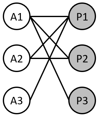
Exercise 14

Write the equations for animal species 2 and 3 following the examples provided below for plant species 1 and 3. $$ \frac{dN_1^P}{dt} = (r_1^P - s_1^P N_1^P + \alpha_{11}^A N_1^A + \alpha_{12}^A N_2^A + \alpha_{13}^A N_3^A) N_1^P $$ $$ \frac{dN_3^P}{dt} = (r_3^P - s_3^P N_3^P + \alpha_{31}^A N_1^A) N_3^P $$

NOTE: We will work together in class to understand the summation and connect it to the network!

Now that we have understood together the summation and its connection to the plant-pollinator network, we will see how the computer can help us with building the system of differential equations using matrices.

Multi-species Lotka-Volterra mutualism model

Let’s start by saving the matrix representing the toy network

interactionMatrix = matrix(c(1, 1, 1, 1, 1, 0, 1, 0, 0), 
                           nrow = 3, byrow = TRUE)
print(interactionMatrix)

We will now generate a matrix with alphas drawn from a uniform random distribution for all P x A combinations for lack of a better parameter choice (i.e. we don’t have empirical estimates of mutualism strengths). For that, we will extract the number of plants and pollinators from the adjacency matrix and use them as input for the function that draws values from random uniform distribution in R (runif()):

# Get the number of rows (plant species) and columns (animal species) of the matrix encoding the plant-pollinator network (interactionMatrix)
num_plants <- nrow(interactionMatrix)
num_animals <- ncol(interactionMatrix)

# Number of interactions
L=num_plants*num_animals

# Set the mean and variance of the random uniform distribution
mean_alpha <- 0.5
variance <- 0.2

# Generate the 3x3 matrix with values from a uniform random distribution
matrix_alpha <- runif(L, mean_alpha - variance/2, mean_alpha + variance/2)
matrix_alpha <- matrix(matrix_alpha, nrow = num_plants, byrow = TRUE)

# Print the matrix
print(matrix_alpha)

To illustrate how we will use matrix operations to build the multi-species model, we will start by showing what you obtain when multiplying element-by-element a randomly generated matrix with all possible interaction strengths between plant and animal species (matrix of alphas) with the adjacency matrix that represents the network of plant-pollinator interactions. That is, we obtain the interaction strengths corresponding to the network we are studying: $$ \text{alpha matrix} \odot \text{interaction matrix} $$ $$ =\begin{bmatrix} 0.46 & 0.53 & 0.51 \\ 0.58 & 0.51 & 0.53 \\ 0.41 & 0.58 & 0.46 \end{bmatrix} \odot \begin{bmatrix} 1 & 1 & 1 \\ 1 & 1 & 0 \\ 1 & 0 & 0 \end{bmatrix} $$ $$ =\begin{bmatrix} 0.46 & 0.53 & 0.51 \\ 0.58 & 0.51 & 0 \\ 0.41 & 0 & 0 \end{bmatrix} $$ Note that this alpha matrix might not be the one you generated as the code chunk above generate a new random matrix each time. Its purpose is only to illustrate what happens when you multiply element-by-element two matrices, especially when one has ones and zeroes (i.e., the adjacency matrix)

The R code that performs such multiplication is

# Multiplying element-by-element the interaction matrix and the matrix with interaction strengths:
alpha_realized <- interactionMatrix * matrix_alpha

print("Interaction strengths realized:")
print(alpha_realized)

We will now calculate the sum of mutualistic effects that each animal population provides to each plant population. For example, such sum for plant species 1 is: $$ \alpha_{11}^{A} N_1^{A} + \alpha_{12}^{A} N_2^{A} + \alpha_{13}^{A} N_3^{A} $$ To calculate such contribution to plant growth, we will first randomly generate the abundance of each animal population:

# Set the mean and variance for uniform random distribution
mean_N <- 0.5
var_N <- 0.1

# Draw animal abundances from uniform random distribution
N_A <- runif(num_animals, mean_N - var_N/2, mean_N + var_N/2)

# Ensure N_A is a matrix for proper matrix multiplication (only in R, Matlab allow multiplying matrices and vectors as one does mathmatically)
N_A_matrix <- matrix(N_A, nrow = length(N_A), ncol = 1)

print("Vector of animal abundances:")
print(N_A_matrix)

To illustrate what the following code will do mathematically, here is an example of the matrix shown above with the realized alphas multiplying the vector of animal abundances, which gives us the benefits to population growth each plant species gets from their interactions with pollinators: $$ \begin{bmatrix} 0.46 & 0.53 & 0.51 \\ 0.58 & 0.51 & 0 \\ 0.41 & 0 & 0 \end{bmatrix} \times \begin{bmatrix} 0.52 \\ 0.46 \\ 0.54 \end{bmatrix} $$ $$ =\begin{bmatrix} 0.46 \times 0.52 + 0.53 \times 0.46 + 0.51 \times 0.54 \\ 0.58 \times 0.52 + 0.51 \times 0.46 + 0 \\ 0.41 \times 0.52 + 0 + 0 \end{bmatrix} $$ $$ =\begin{bmatrix} 0.76 \\ 0.54 \\ 0.21 \end{bmatrix} $$

# Summed effects on plants across the pollinators that visit them
effects_onP<-(interactionMatrix * matrix_alpha) %*% N_A_matrix

print("Summed effects of pollinators on plants:")
print(effects_onP)

Now that we understand the basics, we will generate all the parameters and initial conditions to run the multi-species model:


# Set the mean and variance for random distribution
mean_r <- 0.3
var_r <- 0.1

mean_s <- 0.2
var_s <- 0.1

mean_N <- 0.5
var_N <- 0.1

# Generate intrinsic growth rates and self-limitations vectors for plants and animals with values from their respective uniform random distributions
rP <- runif(num_plants, mean_r - var_r/2, mean_r + var_r/2)
rA <- runif(num_animals, mean_r - var_r/2, mean_r + var_r/2)
sP <- runif(num_plants, mean_s - var_s/2, mean_s + var_s/2)
sA <- runif(num_animals, mean_s - var_s/2, mean_s + var_s/2)

# Generate initial conditions vectors for plants and animals with values from their respective uniform random distributions
N_P <- runif(num_plants, mean_N - var_N/2, mean_N + var_N/2)
N_A <- runif(num_animals, mean_N - var_N/2, mean_N + var_N/2)

# Ensure N_P and N_A are matrices for proper matrix multiplication (only in R, Matlab allow multiplying matrices and vectors as one does mathmatically)
N_P_matrix <- matrix(N_P, nrow = length(N_P), ncol = 1)
N_A_matrix <- matrix(N_A, nrow = length(N_A), ncol = 1)

# Define the variables for output
variables <- list(
  "Plant intrinsic growth rates:" = rP,
  "Animal intrinsic growth rates:" = rA,
  "Plant self-limitations:" = sP,
  "Animal self-limitations:" = sA,
  "Plant initial abundances:" = N_P_matrix,
  "Animal initial abundances:" = N_A_matrix
)

# Print the variables with spacing
for (variable_name in names(variables)) {
  cat(variable_name, "\n")
  print(variables[[variable_name]])
  cat("\n")
}

Now, we form the equations and obtain the population growth rate at the initial time step:

# Equations
dPdt <- (rP - sP * N_P_matrix + (matrix_alpha * interactionMatrix) %*% N_A_matrix) * N_P_matrix

dAdt <- (rA - sA * N_A_matrix + (matrix_alpha * interactionMatrix) %*% N_P_matrix) * N_A_matrix

# Printing results
print("dN_i^P/dt:")
print(dPdt)

cat("\n")

print("dN_i^A/dt:")
print(dAdt)

So, all together the code to run the multi-species model is:

# Load matrix:
interactionMatrix = matrix(c(1, 1, 1, 1, 1, 0, 1, 0, 0), nrow = 3, byrow = TRUE)

# Initialize variables
time_steps <- 12
results <- matrix(0, nrow = time_steps, ncol = 2)

# Get the number of rows (plant species) and columns (animal species) of the matrix encoding the plant-pollinator network (interactionMatrix)
num_plants <- nrow(interactionMatrix)
num_animals <- ncol(interactionMatrix)

# Number of interactions
L=num_plants*num_animals


# Set the mean and variance for uniform random distributions
mean_alpha <- 0.5
var_alpha <- 0.2

mean_r <- 0.3
var_r <- 0.1

mean_s <- 0.2
var_s <- 0.1

mean_N <- 0.5
var_N <- 0.1

# Generate the 3x3 matrix with values from a uniform random distribution
matrix_alpha <- runif(L, mean_alpha - var_alpha/2, mean_alpha + var_alpha/2)
matrix_alpha <- matrix(matrix_alpha, nrow = num_plants, byrow = TRUE)

# Generate intrinsic growth rates and self-limitations vectors for plants and animals with values from their respective uniform random distributions
rP <- runif(num_plants, mean_r - var_r/2, mean_r + var_r/2)
rA <- runif(num_animals, mean_r - var_r/2, mean_r + var_r/2)
sP <- runif(num_plants, mean_s - var_s/2, mean_s + var_s/2)
sA <- runif(num_animals, mean_s - var_s/2, mean_s + var_s/2)

# Generate initial conditions vectors for plants and animals with values from their respective uniform random distributions
N_P <- runif(num_plants, mean_N - var_N/2, mean_N + var_N/2)
N_A <- runif(num_animals, mean_N - var_N/2, mean_N + var_N/2)

# Ensure N_P and N_A are matrices for proper matrix multiplication (only in R, Matlab allow multiplying matrices and vectors as one does mathmatically)
N_P_matrix <- matrix(N_P, nrow = length(N_P), ncol = 1)
N_A_matrix <- matrix(N_A, nrow = length(N_A), ncol = 1)

for (i in 1:time_steps) {
  # Calculate dP/dt and dA/dt
  dPdt <- (rP - sP * N_P_matrix + (matrix_alpha * interactionMatrix) %*% N_A_matrix) * N_P_matrix
  dAdt <- (rA - sA * N_A_matrix + (matrix_alpha * interactionMatrix) %*% N_P_matrix) * N_A_matrix
  
  # Update N_P_matrix and N_A_matrix
  N_P_matrix <- N_P_matrix + dPdt
  N_A_matrix <- N_A_matrix + dAdt
  
  # Store the results
  results[i, ] <- c(N_P_matrix[1], N_A_matrix[1])
}

# Print the results
print(results)

Exercise 15

Play with the parameters of the model (i.e., the mean of the random distributions) to obtain different results based on what you learned from the model of two species. Can you obtain different mode behaviors such as populations growing to infinity or extinctions? You will need to also change the number of time steps to see the different behaviors.

Exercise 16

How do you think the addition of saturating benefits would change the results of this model? See the work by Okuyama & Holland 2008 (Ecology Letters, 11: 208–216) who modified this model by incorporating a hyperbolic functional response to represent that the beneﬁts to mutualists saturate with the densities of mutualistic species with which they interact.

Consumer-resource

For about 70 years, theoretical research analyzing the population dynamics of mutualisms roughly only assumed Lotka-Volterra-type models (sensu Valdovinos 2019) to conduct their studies (e.g., Kostitzin 1934; Gause and Witt 1935; Vandermeer and Boucher 1978; Wolin and Lawlor 1984; Bascompte et al. 2006; Okuyama and Holland 2008; Bastolla et al. 2009). Those models represent mutualistic relationships as direct positive effects between species using a (linear or saturating) positive term in the growth equation of each mutualist that depends on the population size of its mutualistic partner. While this research increased our understanding of the effects of facultative, obligate, linear, and saturating mutualisms on the long-term stability of mutualistic systems, a more sophisticated understanding of their dynamics (e.g., transients) and of phenomena beyond the simplistic assumptions of the Lotka-Volterra-type models was extremely scarce. A more mechanistic consumer-resource approach to mutualisms was proposed by Holland and colleagues (Holland et al. 2005; Holland and DeAngelis 2010) and further developed by Valdovinos et al. (2013, 2016, 2018). This approach decomposes the net effects assumed to be always positive by Lotka-Volterra-type models into the biological mechanisms producing those effects, including the gathering of resources and exchange of services.

The key advance of the consumer-resource model developed by Valdovinos et al. (2013) is separating the dynamics of the plants’ vegetative biomass from the dynamics of the plants’ floral rewards. This separation allows (i) tracking the depletion of floral rewards by pollinator consumption, (ii) evaluating exploitative competition among pollinator species consuming the floral rewards provided by the same plant species, and (iii) incorporating the capability of pollinators (adaptive foraging) to behaviorally increase their foraging effort on the plant species in their diet with more floral rewards available. Another advance of this model is incorporating the dilution of conspecific pollen carried by pollinators, which allows tracking competition among plant species for the quality of pollinator visits.

A conceptual diagram of the model, focused on the consumer-resource part is:

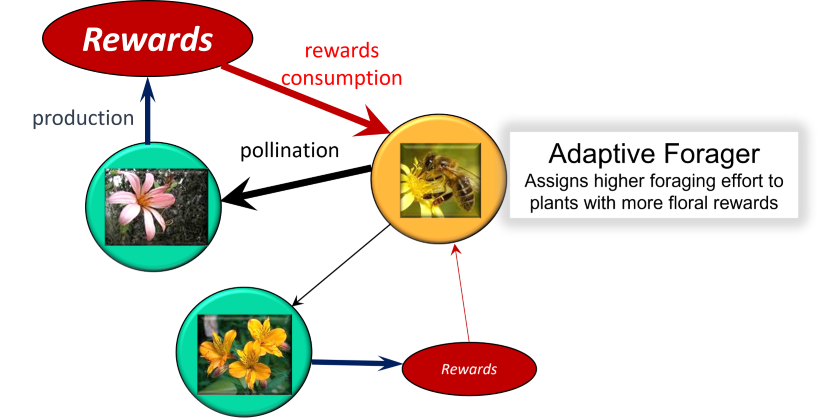
This model defines the population dynamics (over time t) of each plant (Eq. 1) and pollinator (Eq. 2) species of the network, as well as the dynamics of floral rewards (Eq. 3) of each plant species, and the foraging effort (Eq. 4) that each pollinator species (per capita) assigns to each plant species as follows:

$$ \frac{{dp_i}}{{dt}} = \gamma_i \sum_{j \in A_i} e_{ij} \sigma_{ij} V_{ij} - \mu_i^P p_i \quad (Eq. 1) $$

$$ \frac{{da_j}}{{dt}} = \sum_{i \in P_j} c_{ij} V_{ij} b_{ij} \frac{{R_i}}{{p_i}} - \mu_j^A a_j \quad (Eq. 2) $$

$$ \frac{{dR_i}}{{dt}} = \beta_i p_i - \phi_i R_i - \sum_{j \in A_i} V_{ij} b_{ij} \frac{{R_i}}{{p_i}} \quad (Eq. 3) $$

$$ \frac{{d\alpha_{ij}}}{{dt}} = G_j \alpha_{ij} \left( c_{ij} \tau_{ij} b_{ij} R_i - \sum_{k \in P_j} \alpha_{kj} c_{kj} \tau_{kj} b_{kj} R_k \right) \quad (Eq. 4) $$

And the biological processes and assumptions of this model are:

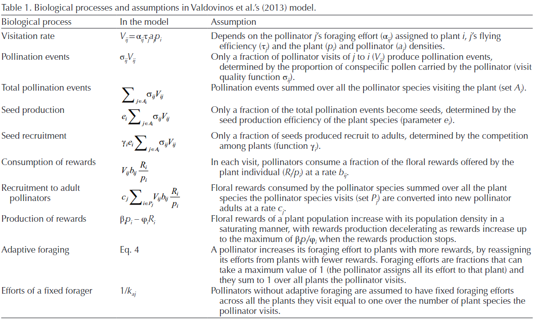
Table 1 from Valdovinos et al 2023, Oikos

Despite its apparent complexity, this model provides clear and consistent results, which are:

Generalist pollinators have more available food (floral rewards) to them than specialist pollinators, which results in generalist pollinator species exhibiting much higher abundances than specialist pollinator species, particularly in nested networks and in networks without adaptive foraging (AF, see point 4).
Generalist plants receive more visits than their specialist counter-parts but this does not necessarily results in generalist plant species having higher abundances than specialist plants because competition for seed recruitment to adults (not pollination) determines the final abundance of plants (see point 6, below).
Generalist plants receive much higher quality of visits than specialist plants in highly nested and moderately connected networks (typical of empirical networks) because they receive high-quality of visits by specialist pollinator species, which allow generalist plant species to persist. Conversely, specialist plant species typically go extinct in these networks without adaptive foraging (AF) because they receive very low quality of visits by generalist pollinators carrying very diluted conspecific pollen. This is because generalist pollinators carry high heterospecific pollen loads when they do not exhibit adaptive foraging in highly nested networks.
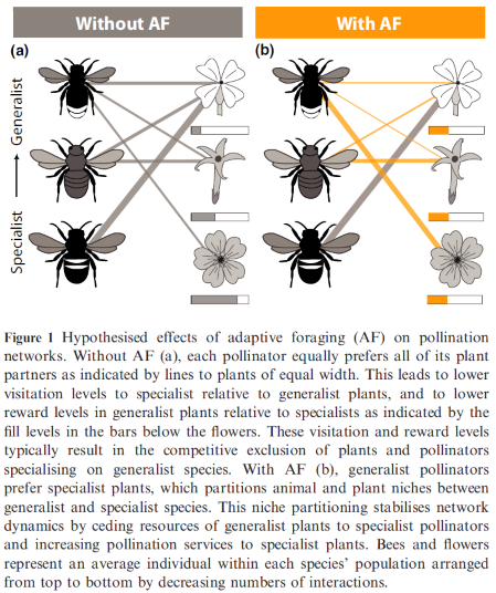
Pollinators with adaptive foraging (AF) assign higher per-capita foraging efforts to specialist plants in highly nested and moderately connected networks, because those plants have more rewards available to them (less consumed) than generalist plants that are much more visited. This re-distribution of foraging efforts causes niche partitioning of floral rewards among pollinator species and of pollination services among plant species, which allows specialist species of plants and pollinators to coexist with their generalist counter-parts. That is, after this re-distribution of foraging efforts by generalist pollinators from generalist to specialist plants, specialist pollinators have more floral rewards available to them because generalist pollinators are not depleting the rewards of generalist plants. Similarly, specialist plants persist because they receive much higher quality of visits of generalist pollinator focusing their foraging efforts on specialist plants and, therefore, carry mostly their conspecific pollen. This niche partitioning is illustrated by the figure below published in Valdovinos et al 2016 (Ecology Letters):

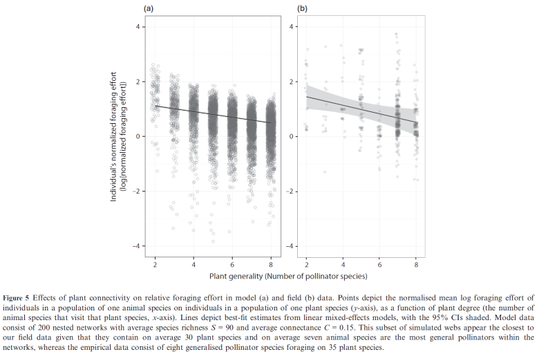
Which Valdovinos et al 2016 also finds for 8 species of bumblebees in RMBL, see panel (a) for empirical data and panel (b) for model results showing that pollinators, in a per-capita basis, prefer specialist (i.e., those visited by one or a few pollinator species) over generalist plants:

Plant species exhibit two stable attractors, they either go to their carrying capacity reduced by inter-specific competition or they go extinct. Plant final abundances when they persist is determined by their intra-specific and inter-specific competition for other resources that are not pollination, which determine seed recruitment to adults. Whether a plant population goes to one or the other attractor depends on the plant population receiving a minimum of quality of visits from their pollinators, which occurs (or not) during the model transient dynamics. This is in fact a threshold dynamics which is common to all models of obligate mutualisms (Hale & Valdovinos 2021, Ecology & Evolution).
Competition for resources that determine seed recruitment to adults (not pollination) affects the final plant abundance when the minimum quality of visits is reached and the plant population persists. That is, pollination determines whether the plant population persists or not, but not its final abundance when the plant persists. In fact, the plant abundance at equilibrium is $p_i \approx \frac{K_l}{w_i}$ where $K_l = 1 - \sum_{l \neq i} u_l p_l$ , $w_i$ is intra-specific and $u_l$ inter-specific competition for recruitment.
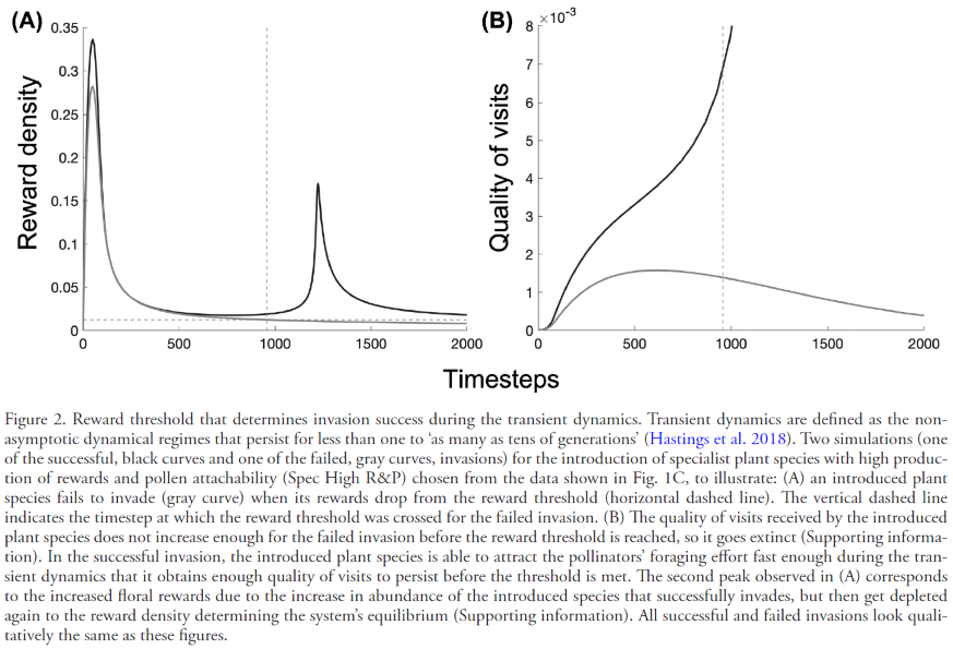
If the floral rewards of a plant population drop below the R* needed for pollinators to persist, the plant population goes extinct because pollinators stop visiting it. Floral rewards available to pollinators determine whether a plant population attracts fast enough the pollinator foraging efforts during the transient dynamics to meet its minimum quality of visits to persist. Dropping below R* starts a non-reversible process to plant extinction, which can occur when a plant receives too many low-quality visits that deplete the rewards below R* but do not meet the quality of visits needed for the plant to persist. This behavior of the model can be seen, for example, when a plant species enters the network with very low abundance, which requires the plant to produce more floral rewards than its neighbors to attract the pollinator foraging effort fast enough to receive high quality of visits. Generalist plants at low abundance are the ones that most likely would go extinct via this mechanism, especially in overly-connected networks. An illustration of this behavior can be found in the figure below from Valdovinos et al 2023, which studies plan invasions:

This R* keeps the meaning given by Tilman but results from an ideal-free-distribution process, in which pollinators keep changing their foraging efforts until the rewards of all plant populations reach the same value, R*, after which foraging efforts of pollinators stop changing and the model dynamics cruises to its equilibrium.

Final thoughts

We hope that after these three days you have learned something new in terms of empirical and theoretical research in plant-pollinator systems and how to integrate both types of research. During the first day, we learned the basics of network structure and how to manipulate empirical data to build plant-pollinator networks, and analyze them. During the second day, we learned about statistical approaches to analyze species interactions which can provide more detailed understanding to our plant-pollinator and network studies. During the third day, we went back to dynamics studied mathematically from simple and phenomenological models of one species to phenomenological models of networks to a more mechanistic consumer-resource model of plant-pollinator networks.

We wish you the best in your next scientific steps and that you can integrate some of what you learned in these three days into your research.

Readings

Hale, K.R.S., & Valdovinos, F.S. (2021) Ecological theory of mutualism: Qualitative patterns in two-species population models. Ecology and Evolution, 00, 1-21.

Okuyama, T., & Holland, J. N. (2008). Network structural properties mediate the stability of mutualistic communities. Ecology letters, 11(3), 208-216.

Valdovinos, F.S., Moisset de Espanés, P., Flores J.D, Ramos-Jiliberto, R. (2013) Adaptive foraging allows the maintenance of biodiversity of pollination networks. Oikos 122: 907-917.

Valdovinos, F.S., Brosi, B.J., Briggs, H.M., Moisset de Espanés, P., Ramos-Jiliberto, R., Martinez, N.D. (2016). Niche partitioning due to adaptive foraging reverses effects of nestedness and connectance on pollination network stability. Ecology Letters, 19, 1277-1286.

Valdovinos, F.S. (2019) Mutualistic Networks: Moving closer to a predictive theory. Ecology Letters, 22, 1517-1534, DOI:10.1111/ele.13279

Valdovinos, F.S. & Marsland III, R. (2021) Niche theory for mutualism: A graphical approach to plant-pollinator network dynamics. The American Naturalist, 197, 393-404.

Valdovinos, F. S., Dritz, S., & Marsland III, R. (2023). Transient dynamics in plant-pollinator networks: Fewer but higher quality of pollinator visits determines plant invasion success. Oikos. https://doi.org/10.1111/oik.09634

Vandermeer, J. H., & Goldberg, D. E. (2013). Population ecology: first principles. Princeton University Press. pp 225-238.

This is not just an analogy! In fact, for certain systems we can determine what this landscape (defined by the system potential $\phi = -\int_{-\infty}^{\infty} \frac{dN}{dt} dN$) actually looks like quantitatively. ↩︎
We have only a single eigenvalue because we have only a single variable. Later, for systems with $n$ variables, we will have $n$ eigenvalues. ↩︎
What counts as “sufficiently small” depends on how nonlinear the function is. ↩︎

Last updated on Aug 31, 2024