Of Potential Interest
Supplementary materials
$$ \newcommand{\L}{\mathcal{L}} $$
Model fitting
Probability distributions
Mass vs. density
For discrete probability distributions, $P(O | \theta)$ is typically referred to as a probability mass function. Given the parameter(s) $\theta$, each integer value of an outcome $O$ (i.e. the discrete random variable) has some probability (some “mass”) of occurring.
In contrast, for continuous probability distributions, we instead refer to probability density functions, $f(O | \theta)$. That’s because the probability of any specific value of a continuous random variable is zero! Instead, there is only a non-zero probability of the random variable falling within some interval of values. The higher the probability density over that interval, the higher the probability of observing a measurable value from within it.
Likelihood functions
The distinction between probability mass functions and probability density functions is relevant to the likelihood functions for discrete and continuous random variables. For discrete variables (as we will focus on in class), the likelihood of the parameter(s) given the data is equal to the probability of the data given the parameter(s), $$ L(\theta | O) = P(O | \theta). $$ For continuous variables, we maximize the likelihood of the parameter given the data by finding the parameter that maximizes the probability density function. That is, we maximize $$ L(\theta | O) = f(O | \theta). $$
Analytical MLE for Poisson
Given $n$ observations (counts) from a process presumed to be well-described by the Poisson, we have that $$ -\ln \L(\lambda |k) = -\sum_i^n \ln \left (\frac{\lambda^{k_i} e^{-\lambda}}{k_i!} \right) . $$ Remembering that logarithms transform multiplicative processes into additive processes, we can write this as $$ -\ln \L(\lambda |k) = -\sum_i^n \left ( \ln ( \lambda^{k_i} ) + \ln (e^{-\lambda} ) - \ln (k_i!) \right). $$ Since $\ln x^y = y \ln x$ and $\ln e^x = x$, we can simplify this to $$ -\ln \L(\lambda |k) = -\sum_i^n \left ( k_i \ln (\lambda) -\lambda - \ln (k_i!) \right). $$ Distributing the summation, we get $$ -\ln \L(\lambda |k) = -\sum_i^n \left ( k_i \ln \lambda \right) + n\lambda + \sum_i^n \ln (k_i!). $$ Now take the derivative with respect to $\lambda$, set it equal to zero, and solve for $\lambda$: $$ \frac{d -\ln \L(\lambda | k)}{d \lambda} = - \frac{1}{\lambda} \sum_i^n k_i + n = 0 \implies \lambda = \frac{\sum_i^n k_i}{n}, $$ which is the mean value of all the $k_i$ counts!
Our analytically-solved maximum likelihood estimator for $\lambda$, which we will symbolize by $\hat{\lambda}$, is therefore $$ \hat{\lambda} = \frac{\sum_i^n k_i}{n}. $$ This is nothing more than a function, think $\hat{\lambda}(k,n)$, to which we provide a vector of observed $k$ counts and their $n$ number (the vector’s length) as inputs.
Dynamics
Building exponential growth
Population models are focused on rates of births and deaths.
Let’s start out by considering a “closed” population, with no immigration or emigration.
We will set $B$ = births and $D$ = deaths; right now these are terms for the entire population, overall how many births happened and how many deaths happened?
A simple population growth model can be formulated by stating the obvious, starting out with the number of individuals in a population at a defined time that we will call $t$: in the next time period of interest $(t+1)$—for example, one year later—the population size $(N_{t+1})$ will be the current population size $(N_t)$ plus the births $(B)$ that occur between time $t$ and time $t+1$, minus the deaths $(D)$ that occur in that time period.
We can write this model formally as $$ N_{t+1} = N_t + B - D. $$
Thus, if you know the estimated birth and death rates in the coming time period, as well as the current population size, it is easy to calculate what the population size will be for the next time point.
The equation above is what we might call a difference equation: the difference between the population size of our target species at two discrete points in time. For many species, especially those with highly seasonal life cycles like annual plants, it makes sense to model them in discrete time.
At the same time, for species with overlapping generations, especially those that don’t have seasonal reproductive patterns, it makes sense instead to model them in continuous time. It is also mathematically much more tractable to use continuous-time models. For the rest of our discussion of population dynamics, we will focus on continuous-time models.
In thinking about continuous-time models, we move from difference equations like the one presented above to differential equations that are focused on on the change in population size over some continuous swath of time. Calculus is well-suited for this and from here on out, we will use calculus notation to think about the differential equations involved in how population size changes over time, designated as: $\frac{dN}{dt}$. Remember that the $d$ in calculus notation stands for ‘change’: how does population size change as time changes? It can be helpful to think of this as instantaneous change, or change over a very short period of time.
One important thing to remember is that $\frac{dN}{dt}$ is keeping track of the change in population size (not the population size itself), but as we solve these equations to keep track of dynamics, if we have a starting population size then we can track population size over time, because we’re keeping track of how the population changes.
In the case of a closed population, the change in population size is driven only by the births and deaths. In other words,
$$ \frac{dN}{dt} = B - D. $$
Typically, however, $B$ and $D$ are not constants. If they were, you would get a situation where there would be, say, 50 deaths and 52 births, irrespective of if the population is 60 or if the population is 3 billion. That is obviously quite unrealistic.
A more appropriate alternative is to instead assume that birth and death are per-capita (i.e., per-individual) rates, e.g., every individual has two offspring and a 50% chance of dying each year. With per-capita birth and death rates, the total number of births and deaths will typically be very different in a small vs. a large population.
To formalize this, we could call the per-capita birth rate b (lower-case, in contrast to the value for the entire population, $B$) and the death rate d. $b = \frac{B}{N}$ and $d = \frac{D}{N}$ ; in other words, the per-capita rates are the population-level total rates divided by the population size. As such, $B = bN$ and $D = dN$. Thus, you could re-state the equation above as $$ \frac{dN}{dt} = bN - dN. $$
For simplicity, population biologists typically combine the birth and death rates into a single per-capita rate of change in the population. When multiplied by the population size, it tells us how much the population will change in the next time step: if it will go up or down, and by how much. We call this per capita population growth rate. While it is the “growth” rate it is important to note that the per capita growth rate can also be negative—individuals can have a higher probability than dying than giving birth in any moment in time, such that the population can be declining.
Using the equations above, we could derive this per-capita rate of change a few different ways. A relatively simple way to think about it is to take all of the births $(B)$ and all of the deaths $(D)$ in the population and divide those by the number of individuals in the population:
$$ \frac{(B-D)}{N} = b - d = r. $$ Think of $r$ is the net per capita birth/death rate or the intrinsic rate of (net) growth.
We can now use $r$ to formalize the multiplicative model discussed above, which is focused on understanding how population size changes over time (calculus notation) $$ \frac{dN}{dt} = rN. $$
Taylor Series
We can approximate any infinitely-differentiable function (as most dynamical models in ecology are, and most biology is assumed to be described by) to an arbitrary degree of accuracy near some point along it using a Taylor Series. A Taylor Series is an infinite sum of terms involving the function’s derivatives.
(For legibility, we will here write $f’(N)$ to indicate $\frac{d f(N)}{dN}$, $f’’(N)$ to indicate $\frac{d^2 f(N)}{dN}$, etc..)
Specifically, we can express any function $f(N^{*}+x$) describing a population’s response to a perturbation $x$ as
$$ f(N^{*}+x) = \sum_{i=0}^\infty \frac{f^{(i)}(N^{*})}{i!}x^i $$ or, writing out the first four terms, as $$ f(N^{*}+x) = f(N^{*}) + \underbrace{\frac{f’(N^{*})}{1!}n_t^1 + \frac{f’’(N^{*})}{2!} n_t^2 + \frac{f’’’(N^{*}) }{3!}n_t^3 + …}_{\text{h.o.t.}} $$ noting that this is an equality, not an approximation, if the sum goes to infinity.
For (local) stability analysis, we use only the first-order terms to approximate the dynamics of the perturbation, dropping the zeroth term (since $f(N^{*})=0$ by definition) and justifying ignoring all “higher order terms” by assuming the initial magnitude of the perturbation is sufficiently small.
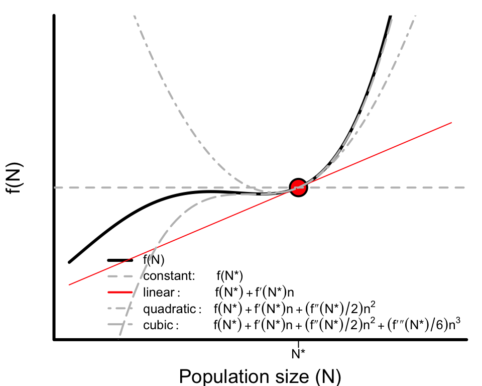
To demonstrate just how well the Taylor Series approximation works, consider the following fourth-order polynomial as an example of some complex function for $dN/dt$
$$ f(N) = -1 + 3.24 N + 5.23 N^2 + 2.8 N^3 + 0.38 N^4 $$ shown in black in the figure below. The red dot represent the point $N^{*}$ at which we are approximating the function, the red line represents our first-order approximation, and the grey lines represent the approximations including successively higher order terms. For a sufficiently small $x$ the slope alone does a very good job. Hopefully it’s clear from this example that what counts is “sufficiently small” depends on how nonlinear the function is.
2-sp Competition
Try it out
Download Dynamics_LV2spComp.R to implement the following code. Play around with the parameter values and initial population sizes to see how they affect the dynamics, whether the two species coexist, or whether one species outcompetes the other.
library(deSolve)
model <- function(t, x, params) {
N1 <- x[1]
N2 <- x[2]
with(as.list(params), {
dN1dt <- r1 * N1 * (1 - N1 / K1 - a12 * N2 / K1)
dN2dt <- r2 * N2 * (1 - N2 / K2 - a21 * N1 / K2)
out <- c(dN1dt, dN2dt)
list(out)
})
}
# Time points at which to evaluate
t <- seq(0, 30, by = 1)
# Starting population sizes at t = 0
xstart <- c(N1 = 0.01,
N2 = 0.01)
# Parameter values
parameters <- c(a12 = 0.5,
a21 = 0.7,
r1 = 1,
r2 = 1,
K1 = 1,
K2 = 1)
# Integrate
out <- as.data.frame(ode(xstart, t, model, parameters))
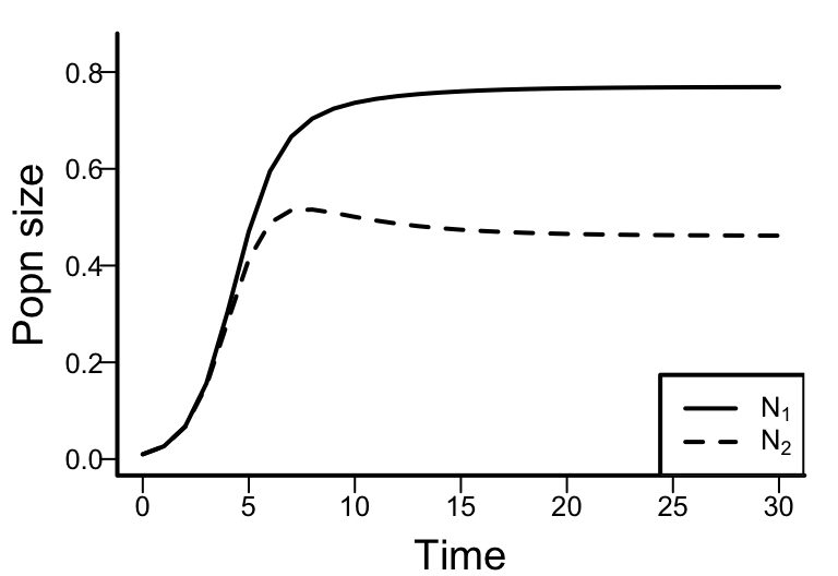
# Plot dynamics over time
plot(out$time,
out$N1,
ylab = 'Popn size',
xlab = 'Time',
type = 'l',
ylim = c(0, max(out$N1, out$N2) * 1.1)
)
lines(out$time,
out$N2,
lty = 2)
legend('bottomright',
legend = c(expression(N[1]), expression(N[2])),
lty = c(1, 2))
Inferences
As you might have observed, in the two-species Lotka-Volterra model, the values of each species’ intrinsic growth rates have no affect on their asymptotic coexistence potential; they affect only the transient dynamics. In fact, the quantitative values of the intraspecific effects (i.e. the carrying capacities) and the interspecific effects don’t affect long-term coexistence either, so long as they satisfy the qualitative requirement that both species experiences weaker interspecific competition than intraspecific competition. That is, if
- $1/K_i = a_{ii} < a_{ij}$ for both species, then they will coexist indefinitely.
Alternatively, if
- $1/K_i = a_{ii} > a_{ij}$ for $i=1$ but not for $i=2$, then species 1 will outcompete species 2;
- $1/K_i = a_{ii} > a_{ij}$ for $i=2$ but not for $i=1$, then species 2 will outcompete species 1.
However, if
- $a_{ii} > a_{ij}$ for both species, then the outcome depends on the species’ initial population sizes.
In this last scenario where both species experience stronger interspecific competition than intraspecific competition (on a per capita scale), the species that wins is the species that starts with the larger population size. That is, we see a so-called priority effect between the alternative final states of the system.
Time-series for all four scenarios are depicted in the left-hand column of the following figures. (Note that, for simplicity, I’ve set $K_1 = K_2 = r_1 = r_2 = 1$.)
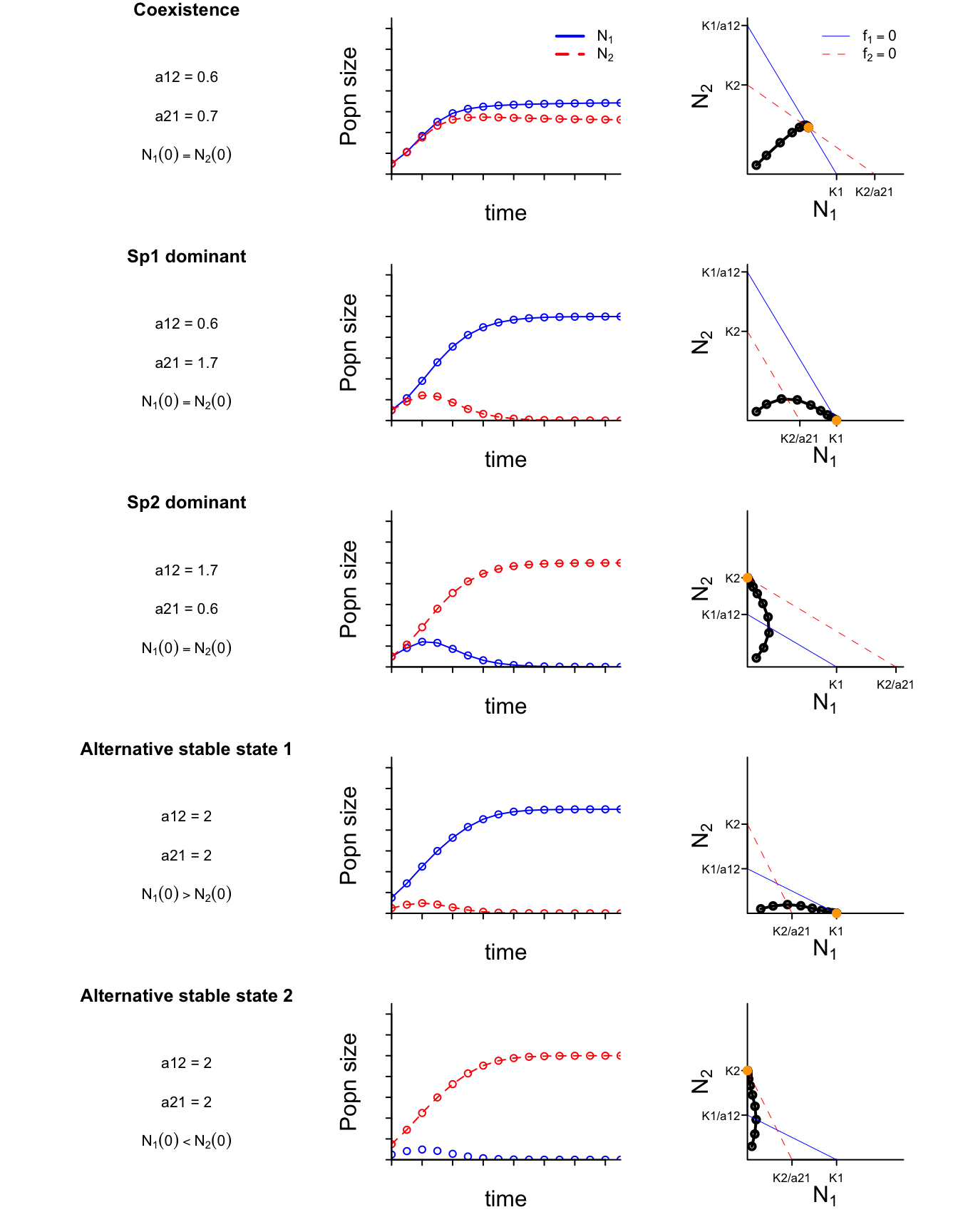
State-space
The the right-hand column of the above figure depicts the same dynamics in state-space, plotting the two state variables (the species’ population sizes, $N_1$ and $N_2$) against each other rather than against time. The orange point depicts the final state of each of the time series. The diagonal lines in each plot are the so-called isoclines (a.k.a. nullclines).
Including the trivial equilibrium (not depicted in the figure), we see four possible steady states from the simulations: ${N_1^{*}, N_2^{*}} = {0, 0}, {N_1, 0}, {0, N_2}, {N_1, N_2}$ Notice that all of the non-trivial steady states are located on one or both isoclines. That’s because each isocline represents the solution to $f_i =\frac{dN_i}{dt}=0$ for one of the species. Where the isoclines intersect we have that both $\frac{dN_i}{dt}=0$ and $\frac{dN_j}{dt}=0$. More specifically, each isocline represents $N_i^{*}$ as a function of $N_j$: $$ N_1^{*} = K_1 - a_{12} N_2 \quad \text{and} \quad N_2^{*} = K_2 - a_{21}N_1 $$ (See next section for the algebra.)
The relative positioning of the isoclines – whether and how they intersect – gives us graphical insight into whether each of the steady states is stable or unstable. For a given fixed valued of $N_j$, perturbations to $N_i$ that cause $N_i$ to go above species $i$’s isocline $N_i^{*}$ will cause $\frac{dN_i}{dt} < 0$ and $N_i$ will decline back to $N_i^{*}$. Conversely, perturbations to $N_i$ that cause $N_i$ to go below species $i$’s isocline $N_i^{*}$ will cause $\frac{dN_i}{dt} > 0$ and $N_i$ will increase back to $N_i^{*}$.
Isoclines
To solve for the isoclines of the two-species Lotka-Volterra competition model.
Step 1: Set $$ f_i = \frac{dN_i}{dt} = 0 $$
Step 2: Solve for $N_i^{*}$ as a function of $N_j$: $$ r_i N_i \left ( 1- \frac{N_i}{K_i} - \frac{a_{ij} N_j}{K_i} \right) =0 $$ $$ r_i N_i - \frac{r_i N_i N_i}{K_i} - \frac{ r_i a_{ij} N_i N_j}{K_i} =0 $$ $$ r_i N_i K_i = r_i N_i N_i + r_i a_{ij} N_i N_j $$ $$ K_i = N_i + a_{ij} N_j $$ $$ N_i^{*} = K_i - a_{ij} N_j $$
2D stability
To evaluate the stability of the 2-dimensional steady state ${N_1^{*}, N_2^{*}}$ will extend the formal “linear stability analysis” that we applied to the 1-dimensional logistic model (#1Dstability). In essence, our criterion for stability will be that $f_i^{'}(N_i^{*}, N_j^{*}) < 0$ for both species, which we will determine using the system’s (two) eigenvalues. Because we’re now considering 2 dimensions, we have to consider not only how $N_i$ responds to a perturbation $x_i$ and how $N_j$ responds to a perturbation $x_j$, but also how $N_i$ responds to $x_j$ and how $N_j$ responds to $x_i$. We’ll therefore be considering a 2x2 matrix of responses.
We’ll again be re-framing to consider not the dynamics of the abundances $N_i$ and $N_j$ but will instead consider the dynamics of the perturbations $x_i$ and $x_j$. That is, we write $$ N_1 = N_1^{*} + x_1 \quad \text{ and } \quad N_2 = N_2^{*} + x_2 $$ such that $$ \frac{dN_1}{dt}=\frac{d(N_1^{*} + x_1)}{dt} = f_1(N_1^{*} + x_1, N_2^{*}+x_2) $$ and $$ \frac{dN_2}{dt}=\frac{d(N_2^{*} + x_2)}{dt} = f_2(N_1^{*} + x_1, N_2^{*}+x_2) $$ Because $N_1^{*}$ and $N_2^{*}$ are constants, the rates of change of $x_1$ and $x_2$ will be the same, thus
$$ \frac{d x_1}{dt} = f_1(N_1^{*} + x_1, N_2^{*}+x_2) \quad \text{ and } \quad \frac{d x_2}{dt} = f_2(N_1^{*} + x_1, N_2^{*}+x_2) $$ The functions $f_1$ and $f_2$ could be very complicated, but we can again approximate them with a Taylor expansion, this time in two dimensions using partial derivatives with respect to each species. That is, we approximate $f_1$ by $$ f_1(N_1^{*} + x_1, N_2^{*}+x_2) \approx $$ $$ f_1(N_1^{*}, N_2^{*}) + \frac{\partial f_1(N_1^{*}, N_2^{*})}{\partial N_1} \cdot x_1 + \frac{\partial f_1(N_1^{*}, N_2^{*})}{\partial N_2} \cdot x_2 + h.o.t. $$ and approximate $f_2$ by $$ f_2(N_1^{*} + x_1, N_2^{*}+x_2) \approx $$ $$ f_2(N_1^{*}, N_2^{*}) + \frac{\partial f_2(N_1^{*}, N_2^{*})}{\partial N_1} \cdot x_1 + \frac{\partial f_2(N_1^{*}, N_2^{*})}{\partial N_2} \cdot x_2 + h.o.t. $$ Since $f_1(N_1^{*}, N_2^{*}) = f_2(N_1^{*}, N_2^{*}) = 0$ by definition, and ignoring all higher order terms (i.e. assuming $x_1$ and $x_2$ are sufficiently small) we arrive at $$ f_1(N_1^{*} + x_1, N_2^{*}+x_2) \approx \frac{\partial f_1(N_1^{*}, N_2^{*})}{\partial N_1} \cdot x_1 + \frac{\partial f_1(N_1^{*}, N_2^{*})}{\partial N_2} \cdot x_2 $$ and $$ f_2(N_1^{*} + x_1, N_2^{*}+x_2) \approx \frac{\partial f_2(N_1^{*}, N_2^{*})}{\partial N_1} \cdot x_1 + \frac{\partial f_2(N_1^{*}, N_2^{*})}{\partial N_2} \cdot x_2 . $$
Community matrix
To make our notation more compact, we can substitute $$ A_{ij} = \frac{\partial f_i(N_1^{*}, N_2^{*})}{\partial N_j} $$ for $i \in {1,2}$ and $j \in {1,2}$.
More explicitly, let
$$
A_{11} = \frac{\partial f_1(N_1^{*}, N_2^{*})}{\partial N_1},
$$
$$
A_{12} = \frac{\partial f_1(N_1^{*}, N_2^{*})}{\partial N_2},
$$
$$
A_{22} = \frac{\partial f_2(N_1^{*}, N_2^{*})}{\partial N_2},
$$
and
$$
A_{21} = \frac{\partial f_2(N_1^{*}, N_2^{*})}{\partial N_1}
$$
We can therefore write our equations for $\frac{d x_1}{dt}$ and $\frac{d x_2}{dt}$ as
$$
\frac{d x_1}{dt} = f_1(N_1^{*} + x_1, N_2^{*}+x_2) \approx A_{11} \cdot x_1 + A_{12} \cdot x_2
$$
and
$$
\frac{d x_2}{dt} = f_2(N_1^{*} + x_1, N_2^{*}+x_2) \approx A_{21} \cdot x_1 + A_{22} \cdot x_2.
$$
We can then represent the two equations even more compactly in matrix form as
$$
\begin{bmatrix}
\frac{dx_1}{dt} \\
\frac{dx_2}{dt}
\end{bmatrix}
\approx
\begin{bmatrix}
A_{11} & A_{12} \\
A_{21} & A_{22}
\end{bmatrix}
\cdot
\begin{bmatrix}
x_1 \\
x_2
\end{bmatrix}
$$
or even more compactly with
$$
\frac{d \textbf{x}}{dt} = \textbf{A} \textbf{x}
$$
where column vector
$$
\textbf{x} =
\begin{bmatrix}
\frac{dx_1}{dt} \\
\frac{dx_2}{dt}
\end{bmatrix}
$$
and matrix
$$
\textbf{A} = \begin{bmatrix}
A_{11} & A_{12} \\
A_{21} & A_{22}
\end{bmatrix}.
$$
The matrix $\textbf{A}$ is commonly referred to as the Community Matrix.1 Each element may be interpreted as an interaction strength in that it describes how a small perturbation to the species in column $j$ affects the population growth rate of the species in row $i$ (with the abundance of all other species in an $n>2$ species system held constant).
Eigenvalues
The eigenvalues of the Community Matrix hold all the information we need to determine the local stability of the steady state.
Eigenvalues can have both real and so-called imaginary parts. The real parts tell us about the local stability. The imaginary parts tell us about the periodicity of the dynamics.
| Criterion | Eigenvalues ($\lambda_i$) |
|---|---|
| (1) | $Re(\lambda_i)< 0$ for all $i$ |
| (2) | $Re(\lambda_i)> 0$ for all $i$ |
| (3) | $Re(\lambda_i) = 0$ for all $i$ |
| (4) | $Re(\lambda_i)< 0$ for some $i$ |
| $(i)$ | $Im(\lambda_i) = 0$ for all $i$ |
| $(ii)$ | $Im(\lambda_i) \neq 0$ for some $i$ |
Criterion 1 reflects the situation where the steady state is at the bottom of a bowl; all perturbations decays exponentially towards zero, so we have stable coexistence.
Criterion 2 reflects the situation where the steady state is at the top of an inverted bowl; all perturbations grow exponentially, so coexistence is unstable.
Criterion 3 reflects a completely flat system potential surface; any perturbation will persist at its initial value, so coexistence is neutrally stable.
Criterion 4 reflects (potential) stability in some dimensions (for some species) but not all, so coexistence is unstable.
Criteria i and ii tells us about how the perturbation decays or grows (e.g., decaying monotonically or with decaying oscillations).
Most of the time we don’t care about whether oscillations occur, only whether coexistence is stable or not. For that we only care about the real parts of the eigenvalues. In fact, note that Criterion 1 is also satisfied by having the dominant eigenvalue (the maximum and most positive eigenvalue) be negative.
Try it
R can do only very limited manipulation of symbolic expressions, but it does have the eigen() function to determine the eigenvalues of a numeric matrix.
# Specify the community matrix
A = matrix( c( -1,   -0.5,
               -0.6, -1.  ),
            byrow = TRUE,
            nrow = 2)

# Determine its eigenvalues
eigs <- eigen(A)$values

print(A)
##      [,1] [,2]
## [1,] -1.0 -0.5
## [2,] -0.6 -1.0
print(eigs)
## [1] -1.5477226 -0.4522774
print(max(eigs))
## [1] -0.4522774
Session Info
## R version 4.4.1 (2024-06-14)
## Platform: aarch64-apple-darwin20
## Running under: macOS Sonoma 14.5
##
## Matrix products: default
## BLAS:   /Library/Frameworks/R.framework/Versions/4.4-arm64/Resources/lib/libRblas.0.dylib
## LAPACK: /Library/Frameworks/R.framework/Versions/4.4-arm64/Resources/lib/libRlapack.dylib;  LAPACK version 3.12.0
##
## locale:
## [1] en_US.UTF-8/en_US.UTF-8/en_US.UTF-8/C/en_US.UTF-8/en_US.UTF-8
##
## time zone: America/Los_Angeles
## tzcode source: internal
##
## attached base packages:
## [1] stats     graphics  grDevices utils     datasets  methods   base
##
## other attached packages:
## [1] deSolve_1.40
##
## loaded via a namespace (and not attached):
##  [1] digest_0.6.37     R6_2.5.1          bookdown_0.40     fastmap_1.2.0
##  [5] xfun_0.47         blogdown_1.19     cachem_1.1.0      knitr_1.48
##  [9] htmltools_0.5.8.1 rmarkdown_2.28    lifecycle_1.0.4   cli_3.6.3
## [13] sass_0.4.9        jquerylib_0.1.4   compiler_4.4.1    highr_0.11
## [17] rstudioapi_0.16.0 tools_4.4.1       evaluate_0.24.0   bslib_0.8.0
## [21] yaml_2.3.10       jsonlite_1.8.8    rlang_1.1.4
-
When matrix $\textbf{A}$ is not evaluated at a steady state it is formally referred to as a Jacobian matrix. ↩︎